`exo_k.atm`

@author: jeremy leconte

This module contain classes to handle the radiative properties of atmospheres. This alows us to compute the transmission and emission spectra of those atmospheres.

Physical properties of the atmosphere are handled in atm_profile.py.

The nomenclature for layers, levels, etc, is as follows (example with 4 layers; Nlay=4):

-------------------  Model top or first level (plev[0])
- - - - - - - - - -  First atmopheric layer (play[0]=plev[0], tlay[0], xlay[0])

-------------------  plev[1]

- - - - - - - - - -  play[1], tlay[1], xlay[1]

-------------------  plev[2]

- - - - - - - - - - play[2], tlay[2], xlay[2]

-------------------  plev[3]

- - - - - - - - - -  bottom layer (play[Nlay-1]=psurf, tlay[3], xlay[3])
------------------- Surface (plev[Nlev-1=Nlay]=psurf)
///////////////////

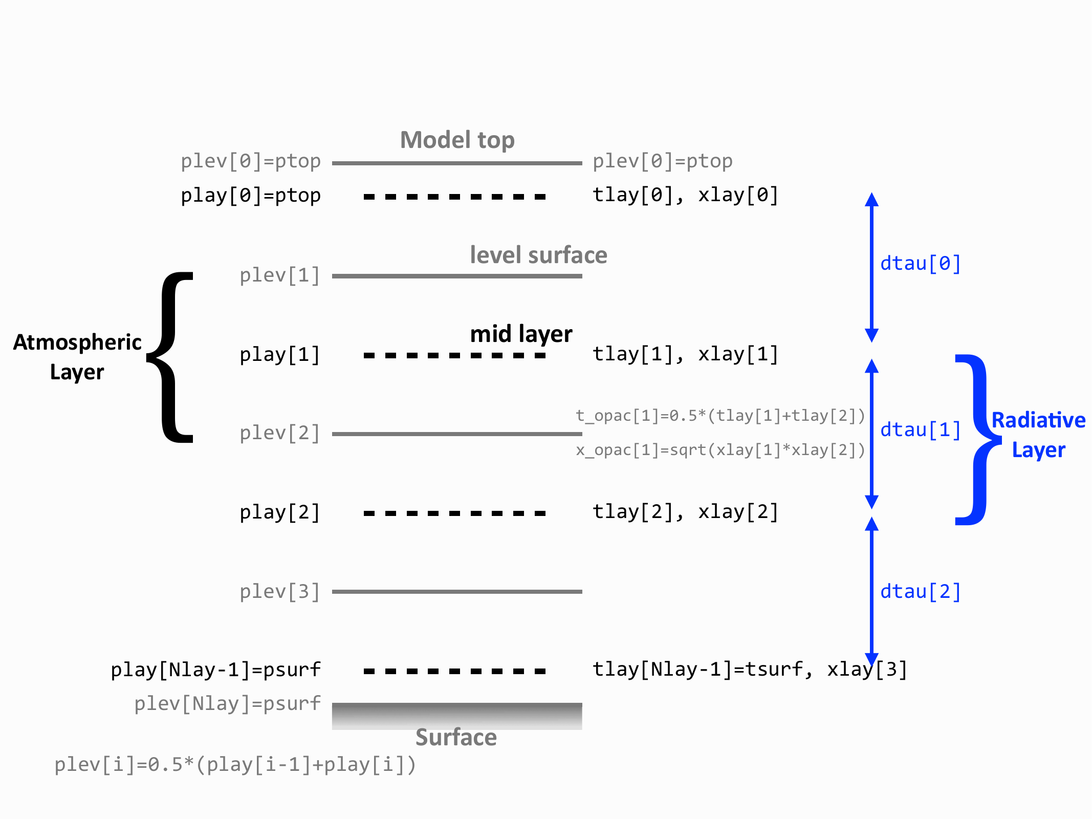
Temperatures (tlay) and volume mixing ratios (xlay) are provided at the mid layer point (play) (Note that this does not mean that this point is the middle of the layer, in general, it is not).

If pressure levels are not specified by the user with logplevel, they are at the mid point between the pressure of the layers directly above and below. The pressure of the top and bottom levels are counfounded with the pressure of the top and bottom mid layer points.

For radiative calculations, the source function (temperature) needs to be known at the boudaries of the radiative layers but the opacity needs to be known inside the radiative layer. For this reason, there are Nlay-1 radiative layers and they are offset with respect to atmospheric layers. Opacities are computed at the center of those radiative layers, i.e. at the pressure levels. The temperature is interpolated at these levels with an arithmetic average. Volume mixing ratios are interpolated using a geometric average.

Module Contents

class exo_k.atm.Atm(k_database=None, cia_database=None, a_database=None, wn_range=None, wl_range=None, internal_flux=0.0, rayleigh=False, flux_top_dw=0.0, Tstar=5570.0, albedo_surf=0.0, wn_albedo_cutoff=5000.0, **kwargs)[source]

Bases: exo_k.atm_profile.Atm_profile

Class based on Atm_profile that handles radiative trasnfer calculations.

Radiative data are accessed through the gas_mix.Gas_mix class.

Initialization method that calls Atm_Profile().__init__(**kwargs) and links to Kdatabase and other radiative data.

set_k_database(k_database=None)[source]

Change the radiative database used by the Gas_mix object handling opacities inside Atm.

See gas_mix.Gas_mix.set_k_database for details.

Parameters:: k_database (Kdatabase object) – New Kdatabase to use.

set_cia_database(cia_database=None)[source]

Change the CIA database used by the Gas_mix object handling opacities inside Atm.

See gas_mix.Gas_mix.set_cia_database for details.

Parameters:: cia_database (CIAdatabase object) – New CIAdatabase to use.

set_a_database(a_database=None)[source]

Change the Aerosol database used by the Aerosols object handling aerosol optical properties.

See aerosols.Aerosols.set_a_database for details.

Parameters:: a_database (Adatabase object) – New Adatabase to use.

set_spectral_range(wn_range=None, wl_range=None)[source]

Sets the spectral range in which computations will be done by specifying either the wavenumber (in cm^-1) or the wavelength (in micron) range.

See gas_mix.Gas_mix.set_spectral_range for details.

set_incoming_stellar_flux(flux_top_dw=None, Tstar=None, stellar_spectrum=None, **kwargs)[source]

Sets the stellar incoming flux integrated in each wavenumber channel.

Important

The normalization is such that the flux input is exactly flux_top_dw whatever the spectral range used.

Parameters:

flux_top_dw (Optional[float]) – Bolometric Incoming flux (in W/m^2).
Tstar (Optional[float]) – Stellar temperature (in K) used to compute the spectral distribution of incoming flux using a blackbody.
stellar_spectrum (Optional[exo_k.util.spectrum.Spectrum]) – Spectrum of the star in units of per wavenumber. The specific units do not matter as the overall flux will be renormalized.

set_internal_flux(internal_flux)[source]: Sets internal flux from the subsurface in W/m^2

set_surface_albedo(albedo_surf=None, wn_albedo_cutoff=None, **kwargs)[source]

Sets the value of the mean surface albedo.

Parameters:

albedo_surf (float) – Effective visible surface albedo.
wn_albedo_cutoff (float) – wavenumber value in cm-1 dividing the visible range from the IR range, where the albedo goes from a given value ‘albedo_surf’ to 0.

_setup_albedo_surf_nu()[source]: Compute the value of the mean surface albedo for each wavenumber in an array. If the albedo value is modified, this method needs to be called again. For now, only available with wavenumbers

set_rayleigh(rayleigh=False)[source]

Sets whether or not Rayleigh scattering is included.

Parameters:: rayleigh (bool) –

spectral_integration(spectral_var)[source]

Spectrally integrate an array, taking care of whether we are dealing with corr-k or xsec data.

Parameters:

spectral_var (array, np.ndarray) – array to integrate

Returns:

var: array, np.ndarray: array integrated over wavenumber (and g-space if relevant)

g_integration(spectral_var)[source]

Integrate an array along the g direction (only for corrk)

Parameters:

spectral_var (array, np.ndarray) – array to integrate

Returns:

var: array, np.ndarray: array integrated over g-space if relevant

opacity(rayleigh=None, compute_all_opt_prop=False, wn_range=None, wl_range=None, **kwargs)[source]

Computes the opacity of each of the radiative layers (m^2/molecule).

Parameters:: rayleigh (bool) – If true, the rayleigh cross section is computed in self.kdata_scat and added to kdata(total extinction cross section) If None, the global attribute self.rayleigh is used.

See gas_mix.Gas_mix.cross_section for details.

source_function(integral=True, source=True)[source]

Compute the blackbody source function (Pi*Bnu) for each layer of the atmosphere.

Parameters:

integral (boolean, optional) –
- If true, the black body is integrated within each wavenumber bin.
- If not, only the central value is used. False is faster and should be ok for small bins, but True is the correct version.
source (boolean, optional) – If False, the source function is put to 0 (for solar absorption calculations)

setup_emission_caculation(mu_eff=0.5, rayleigh=None, integral=True, source=True, gas_vmr=None, Mgas=None, aer_reffs_densities=None, **kwargs)[source]: Computes all necessary quantities for emission calculations (opacity, source, etc.)

emission_spectrum(integral=True, mu0=0.5, mu_quad_order=None, dtau_min=1e-13, **kwargs)[source]

Returns the emission flux at the top of the atmosphere (in W/m^2/cm^-1)

Parameters:

integral (boolean, optional) –
- If true, the black body is integrated within each wavenumber bin.
- If not, only the central value is used. False is faster and should be ok for small bins, but True is the correct version.
mu0 (float) – Cosine of the quadrature angle use to compute output flux
mu_quad_order (int) – If an integer is given, the emission intensity is computed for a number of angles and integrated following a gauss legendre quadrature rule of order mu_quad_order.
dtau_min (float) – If the optical depth in a layer is smaller than dtau_min, dtau_min is used in that layer instead. Important as too transparent layers can cause important numerical rounding errors.

Returns:

Spectrum object: A spectrum with the Spectral flux at the top of the atmosphere (in W/m^2/cm^-1)

emission_spectrum_quad(integral=True, mu_quad_order=3, dtau_min=1e-13, **kwargs)[source]

Returns the emission flux at the top of the atmosphere (in W/m^2/cm^-1) using gauss legendre qudrature of order mu_quad_order

Parameters:

integral (boolean, optional) –
- If true, the black body is integrated within each wavenumber bin.
- If not, only the central value is used. False is faster and should be ok for small bins, but True is the correct version.
dtau_min (float) – If the optical depth in a layer is smaller than dtau_min, dtau_min is used in that layer instead. Important as too transparent layers can cause important numerical rounding errors.

Returns:

Spectrum object: A spectrum with the Spectral flux at the top of the atmosphere (in W/m^2/cm^-1)

emission_spectrum_2stream(integral=True, mu0=0.5, method='toon', dtau_min=1e-10, flux_at_level=False, rayleigh=None, flux_top_dw=None, source=True, compute_kernel=False, **kwargs)[source]

Returns the emission flux at the top of the atmosphere (in W/m^2/cm^-1)

Parameters:

integral (boolean, optional) –
- If True, the source function (black body) is integrated within each wavenumber bin.
- If False, only the central value is used. False is faster and should be ok for small bins (e.g. used with Xtable), but True is the most accurate mode.
rayleigh (bool) – Whether to account for rayleigh scattering or not. If None, the global attribute self.rayleigh is used.
mu0 (float) – Cosine of the quadrature angle use to compute output flux
dtau_min (float) – If the optical depth in a layer is smaller than dtau_min, dtau_min is used in that layer instead. Important as too transparent layers can cause important numerical rounding errors.
flux_at_level (bool) – Whether the fluxes are computed at the levels (True) or in the middle of the layers (False). e.g. this needs to be True to be able to use the kernel with the evolution model.
source (bool) – Whether to include the self emission of the gas in the computation.
compute_kernel (bool) – Whether we want to recompute the kernel of the heating rates along with the fluxes.
method (str) – What method to use to computed the 2 stream fluxes. ‘toon’ (default) uses Toon et al. (1989). ‘lmdz’ is based on the same equation, but the implementation is closer to the actual method used in the LMDZ GCM. This mode is not supported anymore and might be broken!

Returns:

Spectrum object: A spectrum with the Spectral flux at the top of the atmosphere (in W/m^2/cm^-1)

compute_kernel(solve_2stream_nu, epsilon=0.01, flux_at_level=False, mu0=0.5, per_unit_mass=True, integral=True, **kwargs)[source]

Computes the Jacobian matrix d Heating[lay=i] / d T[lay=j]

This method should not be called by the user directly. The recompute the kernel, call emission_spectrum_2stream with the option compute_kernel=True.

After the computation, the kernel is stored in self.kernel and the temperature array at wich the kernel has been computed in self.tlay_kernel.

Parameters:

solve_2stream_nu (function) – Name of the function that will be used to compute the fluxes. e.g.: two_stream_toon or two_stream_lmdz
epsilon (float) – The temperature increment used to compute the derivative will be epsilon*self.tlay
flux_at_level (bool) – Whether the fluxes are computed at the levels (True) or in the middle of the layers (False). e.g. this needs to be True to be able to use the kernel with the evolution model.
mu0 (float) – Cosine of the effective zenith angle used in the flux computations.
per_unit_mass (bool) – Whether the heating rates will be normalized per unit of mass (i.e. the kernel values will have units of W/kg/K). If False, kernel in W/layer/K.
integral (bool) – Whether the integral mode is used in flux computations. e.g. this needs to be True to be able to use the kernel with the evolution model.

flux_divergence(per_unit_mass=True, **kwargs)[source]

Computes the divergence of the net flux in the layers (used to compute heating rates).

emission_spectrum_2stream() needs to be ran first.

Parameters:

per_unit_mass (bool) – If True, the heating rates are normalized by the mass of each layer (result in W/kg).

Returns:

H: array, np.ndarray: Heating rate in each layer (Difference of the net fluxes). Positive means heating. The last value is the net flux impinging on the surface + the internal flux.
net: array, np.ndarray: Net fluxes at level surfaces

heating_rate(compute_kernel=False, dTmax_use_kernel=None, **kwargs)[source]

Computes the heating rates and net fluxes in the atmosphere.

Parameters:

compute_kernel (bool) – If True, the kernel (jacobian of the heat rates) is recomputed
dTmax_use_kernel (float) – Maximum temperature difference between the current temperature and the temperature of the last kernel computation before a new kernel is recomputed.

Returns:

H: array, np.ndarray: Heating rate in each layer (Difference of the net fluxes). Positive means heating. The last value is the net flux impinging on the surface + the internal flux.
net: array, np.ndarray: Net fluxes at level surfaces

bolometric_fluxes_2band(flux_top_dw=None, **kwargs)[source]

Computes the bolometric fluxes at levels and heating rates using bolometric_fluxes.

However, the (up, down, net) fluxes are separated in two contributions:

the part emitted directly by the atmosphere (_emis).
the part due to the incoming stellar light (_stell), that can be used to compute the absorbed stellar radiation and the bond_albedo.

We also provide the associated heating rates (H in W/kg)

spectral_fluxes_2band(**kwargs)[source]

Computes the spectral fluxes at levels.

The (up, down, net) fluxes are separated in two contributions:

the part emitted directly by the atmosphere (_emis).
the part due to the incoming stellar light (_stell), that can be used to compute the absorbed stellar radiation and the bond_albedo.

bolometric_fluxes(per_unit_mass=True, **kwargs)[source]

Computes the bolometric fluxes at levels and the divergence of the net flux in the layers (used to compute heating rates).

emission_spectrum_2stream() needs to be ran first.

Parameters:

per_unit_mass (bool) – If True, the heating rates are normalized by the mass of each layer (result in W/kg).

Returns:

up: array, np.ndarray: Upward fluxes at level surfaces
dw: array, np.ndarray: Downward fluxes at level surfaces
net: array, np.ndarray: Net fluxes at level surfaces
H: array, np.ndarray: Heating rate in each layer (Difference of the net fluxes). Positive means heating. The last value is the net flux impinging on the surface + the internal flux.

transmittance_profile(**kwargs)[source]: Computes the transmittance profile of an atmosphere, i.e. Exp(-tau) for each layer of the model. Real work done in the numbafied function path_integral_corrk/xsec depending on the type of data.

transmission_spectrum(normalized=False, Rstar=None, **kwargs)[source]

Computes the transmission spectrum of the atmosphere. In general (see options below), the code returns the transit depth:

\[\delta_\nu=(\pi R_p^2+\alpha_\nu)/(\pi R_{star}^2),\]

where

\[\alpha_\nu=2 \pi \int_0^{z_{max}} (R_p+z)*(1-e^{-\tau_\nu(z)) d z.\]

Parameters:

Rstar (float or astropy.unit object, optional) –
Radius of the host star. If a float is specified, meters are assumed. Does not need to be given here if it has already been specified as an attribute of the Atm object. If specified, the result is the transit depth:

\[\delta_\nu=(\pi R_p^2+\alpha_\nu)/(\pi R_{star}^2).\]
normalized (boolean, optional) –
Used only if self.Rstar and Rstar are None:
- If True, the result is normalized to the planetary radius:
  
  \[\delta_\nu=1+\frac{\alpha_\nu}{\pi R_p^2}.\]
- If False,
  
  \[\delta_\nu=\pi R_p^2+\alpha_\nu.\]

Returns:

array: The transit spectrum (see above for normalization options).

exp_minus_tau()[source]: Sums Exp(-tau) over gauss points

exp_minus_tau_g(g_index)[source]: Sums Exp(-tau) over gauss point

blackbody(layer_idx=-1, integral=True)[source]

Computes the surface black body flux (in W/m^2/cm^-1) for the temperature of layer layer_idx.

Parameters:

int (layer_idx;) – Index of layer used for the temperature.
integral (boolean, optional) –
- If true, the black body is integrated within each wavenumber bin.
- If not, only the central value is used. False is faster and should be ok for small bins, but True is the correct version.

Returns:

Spectrum object: Spectral flux in W/m^2/cm^-1

surf_bb(**kwargs)[source]

Computes the surface black body flux (in W/m^2/cm^-1).

See blackbody for options.

Returns:

Spectrum object: Spectral flux of a bb at the surface (in W/m^2/cm^-1)

top_bb(**kwargs)[source]

Computes the top of atmosphere black body flux (in W/m^2/cm^-1).

See blackbody for options.

Returns:

Spectrum object: Spectral flux of a bb at the temperature at the top of atmosphere (in W/m^2/cm^-1)

contribution_function()[source]

Compute the contribution function \(Cf(P,\lambda) = B(T,\lambda) \frac{d e^\tau}{d \log P}\).

\(\tau\) and \(\log P\) are taken at the mid-layers, the temperature needs to be taken at the level surfaces. For that, we use the computed temperature t_opac[:-1].

The result is not normalized to allow comparison. :returns: Contribution function [W/m^2/str/cm-1].

Shape: (Nlay - 1, Nw).

Return type:: np.ndarray

exo_k.atm

Module Contents

`exo_k.atm`