Modeling atmospheres and their evolution with exo_k: a practical guide
Author: Jeremy Leconte (CNRS/LAB/Univ. Bordeaux)
Since exo_k allows anyone to easily read radiative data and interpolate into them, it seemed silly not to incorporate a module to test this directly in a real-life situation. This is why we implemented the Atm class that will allow you to build atmospheres with any composition, and compute their transmission/emission spectra with any combination of radiative data that the library can handle. It can also compute the radiative heating rates in each atmospheric layer.
But why stop there? Indeed, heating rates allow you to compute the radiative equilibrium of an atmosphere. One thing led to another, and we ended up with a full-fledged atmospheric model able to compute the evolution of an atmosphere in time that accounts for radiation (of course), dry convection, but also moist convection, condensation, turbulent diffusion, etc. This model is encapsulated in the :class:~exo_k.atm_evolution.atm_evol.Atm_evolution class that will be presented below.
See also
The goal of this section is to give you a practical tour of how to use these classes in a realistic setting. If you want more information on the inner workings of the various modules, you can go to the “Principles of atmospheric modeling with Exo_k” page. For details on how to load radiative data and some general features of the library, please go see the tutorial on “Getting started with radiative data”.
Initialization
First, let’s make some common initializations. To install the library, see the ‘Getting Exo_k’ page.
Important
For efficiency reasons, the atmospheric models work with a single unit system, which is the international MKS system. To avoid loading radiative data in another unit system, we encourage you to always use the global setting xk.Settings().set_mks(True) that will automatically do all the conversions for you.
[1]:
import time

import astropy.units as u
import matplotlib.pyplot as plt
import numpy as np

import exo_k as xk

xk.Settings().set_mks(True)
We also set up the generic path toward the radiative data
[2]:
datapath = '../data/'

xk.Settings().set_search_path(datapath + 'xsec', path_type='xtable')
xk.Settings().set_search_path(datapath + 'corrk', path_type='ktable')
xk.Settings().set_search_path(datapath + 'cia', path_type='cia')
xk.Settings().search_path
[2]:
{'ktable': ['/builds/jleconte/exo_k-public/data/corrk'],
 'xtable': ['/builds/jleconte/exo_k-public/data/xsec'],
 'cia': ['/builds/jleconte/exo_k-public/data/cia'],
 'aerosol': ['/builds/jleconte/exo_k-public/tutorials']}
[3]:
# Uncomment the line below if you want to enable interactive plots
#%matplotlib notebook
plt.rcParams["figure.figsize"] = (7, 4)
from cycler import cycler

colors = cycler('color', [plt.cm.inferno(i) for i in np.linspace(0.1, 1, 5)])
plt.rc('axes', axisbelow=True, grid=True, labelcolor='dimgray', labelweight='bold', prop_cycle=colors)
plt.rc('grid', linestyle='solid')
plt.rc('xtick', direction='in', color='dimgray')
plt.rc('ytick', direction='in', color='dimgray')
plt.rc('lines', linewidth=1.5)
The Atm class: An atmospheric radiative-transfer model
Whether you want to test various assumptions (will my resolution be enough, are my initial data adequate, what weights should I use, etc.) or directly simulate the transmission/emission spectrum of a planet, we implemented a simple 1D atmosphere model so that you can do just that.
This revolves around the Atm() class, which defines an atmosphere with Pressure, Temperature, and composition profiles. In essence, we are using the structure of the Gas_mix object and add the additional attributes that make an atmosphere more than just some gas with a given pressure, temperature, and composition: a gravity, a planetary radius, etc.
As Xtable() objects can be used in a Kdatabase(), you can do the equivalent of Line by Line radiative transfer.
If you want to start from very high-res spectra, first load them into a Xtable(), and then into a Database.
See also
Check out Atm and its base class Atm_profile
for details on arguments and options.
Important
Pressure is the primary coordinate used to build the atmospheric profiles (and not altitude). To keep pressure arrays in increasing order, the atmosphere is therefore described from the top down. The first element of each array describes the atmosphere (temperature, composition, etc.) refers to the uppermost layer of the atmosphere. The surface is described by the last element of each array.
Also note that since v1.1.0, there is a new scheme for the computation of atmospheric emission/transmission to improve numerical accuracy. This led to the change of some variable names to instantiate atm objects (Nlev, logplev, and tlev are now Nlay, logplay and tlay).
Loading the radiative data that we will use in our atmospheric model
Molecular absorptions: The Kdatabase
The first thing that we need to do is to create a Kdatabase that will contain the data for all the molecules that we want to include in our atmosphere and for which we have cross sections (whether they are monochromatic cross sections of correlated-k coefficients).
Important
An Atm instance will inherit its spectral range and resolution for the radiative computations from the Kdatabase it is given. So it is important to choose radiative data that cover the wavelength range that you want to model.
As a corollary, even if you want to model an atmosphere for which you have only continuum absorptions (like Rayleigh or Collision Induced Absorptions), you still need to provide a Kdatabase that has at least one molecule in it. If you do not, the model will not be able to know which spectral window to model. We will show later how to turn off the molecular absorptions.
In the example below we will treat a simple examples with only CO2 and H2O. Other gases, if any, will only contribute through continuum absorptions.
[4]:
k_db = xk.Kdatabase(['CO2', 'H2O'], 'R300_0.3-50mu.ktable.SI')
k_db
[4]:
The available molecules are:
CO2->/builds/jleconte/exo_k-public/data/corrk/CO2_R300_0.3-50mu.ktable.SI.h5
H2O->/builds/jleconte/exo_k-public/data/corrk/H2O_R300_0.3-50mu.ktable.SI.h5
All tables share a common spectral grid
All tables share a common logP-T grid
All tables share a common p unit
All tables share a common kdata unit
Important
All tables in the Kdatabase must have the same wavenumber, pressure, temperature (and gauss-point) grids. If this is not the case, refer to the general tutorial to see how to correct that.
Collision induced absorptions
Now we can load CIA data in a CIA_database. If you do not want to include such contributions, do not provide any CIA database when instantiating your Atm object or use cia_database=None.
[5]:
cia_db = xk.CIAdatabase(molecules=['N2', 'H2O', 'H2', 'He'], mks=True)
cia_db
[5]:
The available molecule pairs are:
N2-N2->/builds/jleconte/exo_k-public/data/cia/N2-N2_2011.hdf5
N2-H2->/builds/jleconte/exo_k-public/data/cia/N2-H2_2011.hdf5
H2O-N2->/builds/jleconte/exo_k-public/data/cia/H2O-N2_continuumTurbet_MT_CKD3.3.hdf5
H2O-H2O->/builds/jleconte/exo_k-public/data/cia/H2O-H2O_continuumTurbet_MT_CKD3.3.hdf5
H2-H2->/builds/jleconte/exo_k-public/data/cia/H2-H2_2011.hdf5
H2-He->/builds/jleconte/exo_k-public/data/cia/H2-He_2011.hdf5
All tables do NOT have common spectral grid
You will need to run sample before using the database
Just like with the Kdatabase, all the CIA tables must use the same spectral axis (and the same as the Kdatabase) so we usually need to resample our database on the same grid as follows.
[6]:
cia_db.sample(k_db.wns)
cia_db
[6]:
The available molecule pairs are:
N2-N2->/builds/jleconte/exo_k-public/data/cia/N2-N2_2011.hdf5
N2-H2->/builds/jleconte/exo_k-public/data/cia/N2-H2_2011.hdf5
H2O-N2->/builds/jleconte/exo_k-public/data/cia/H2O-N2_continuumTurbet_MT_CKD3.3.hdf5
H2O-H2O->/builds/jleconte/exo_k-public/data/cia/H2O-H2O_continuumTurbet_MT_CKD3.3.hdf5
H2-H2->/builds/jleconte/exo_k-public/data/cia/H2-H2_2011.hdf5
H2-He->/builds/jleconte/exo_k-public/data/cia/H2-He_2011.hdf5
All tables share a common spectral grid
Rayleigh scattering
For the moment, the data for Rayleigh scattering are hardcoded inside the library. So there is no need to load them. You’ll just have to use the rayleigh=True keyword when instantiating your Atm object to state that you want to account for rayleigh scattering in any subsequent radiative transfer calculation (even for emission calculations).
This behavior can also be changed afterwards with Atm.set_rayleigh(rayleigh=True/False).
Finally, the rayleigh keyword can be used with some methods to locally force the presence/absence of rayleigh scattering.
Building an atmosphere
Simple troposphere/stratosphere parametrization
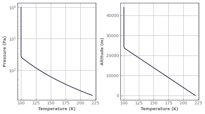
There are several ways to build an atmosphere. If you just want a simple atmospheric structure with an isothermal stratosphere on top of a dry troposphere with a fixed adiabatic gradient, you can just use the following options
[7]:
Nlay = 50  # Number of layers
Tsurf = 220.  # K => Surface temperature
Tstrat = 100.  # K => Temperature of the stratosphere
psurf = 640.  # Pa => Surface pressure
ptop = 1.e0  # Pa => Pressure at the model top
grav = 3.4  # m/s^2 => Surface gravity
rcp = 0.28  # dimless => R/cp
Rp = None  # m => Planetary radius
albedo_surf = 0.2  # m => Surface albedo

composition = {'CO2': 'background', 'H2O': 1.e-6}
# Volume molar concentrations of the various species
# One gas can be set to `background`.
# It's volume mixing ratio will be automatically computed to fill the atmosphere.

atm_mars = xk.Atm(psurf=psurf, ptop=ptop,
                  Tsurf=Tsurf, Tstrat=Tstrat,
                  grav=grav, rcp=rcp, Rp=Rp,
                  albedo_surf=albedo_surf,
                  composition=composition, Nlay=Nlay,
                  k_database=k_db,
                  cia_database=cia_db,  # adding a CIA database entails that CIA will be taken into account.
                  rayleigh=True,  # by default, rayleigh scattering is turned off
                  )
Important
If the sum of the Volume molar concentrations is not equal to one, the rest of the atmosphere is assumed to be transparent and the molar mass of the gas, if needed, is assumed to be equal to the molar mass of the mix you specified (for example, if you specify that your atmosphere is 25% CO2 and 25% H2O, only half of the atmosphere will be radiatively active, but the molar mass will still be about 0.031kg/mol).
Warning
The planetary radius is optional. However, if it is not given, the evolution of gravity with height (in transmission and emission) will not be taken into account.
[8]:
fig, axs = plt.subplots(1, 2, sharey=False, figsize=(7, 4))
atm_mars.plot_T_profile(axs[0], yscale='log')
atm_mars.plot_T_profile(axs[1], use_altitudes=True)
fig.tight_layout()
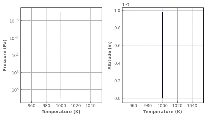
If the stratospheric temperature is set to None, the profile will be isothermal at T=Tsurf.
[9]:
Nlay = 100  # Number of layers
Tsurf = 1000.  # K => Surface temperature
Tstrat = None  # K => Temperature of the stratosphere
psurf = 1.e6  # Pa => Surface pressure
ptop = 1.e-4  # Pa => Pressure at the model top
grav = 10.  # m/s^2 => Surface gravity
rcp = 0.28  # dimless => R/cp
Rp = 1. * u.Rjup  # m => Planetary radius
albedo_surf = 0.  # m => Surface albedo

composition = {'H2': 'background', 'He': 0.09, 'H2O': 1.e-3}

atm_hotjup = xk.Atm(psurf=psurf, ptop=ptop,
                    Tsurf=Tsurf, Tstrat=Tstrat,
                    grav=grav, rcp=rcp, Rp=Rp,
                    albedo_surf=albedo_surf,
                    composition=composition, Nlay=Nlay,
                    k_database=k_db, cia_database=cia_db,
                    rayleigh=True, )

fig, axs = plt.subplots(1, 2, sharey=False, figsize=(7, 4))
atm_hotjup.plot_T_profile(axs[0], yscale='log')
atm_hotjup.plot_T_profile(axs[1], use_altitudes=True)
fig.tight_layout()
Using your own profiles
If you want, you can completely control the profiles you put in your Atm. For this, you just need to provide arrays for logplay, tlay, and the various concentrations.
The atmosphere is defined from the top down so the first value is the top of the atmosphere and the last is the surface.
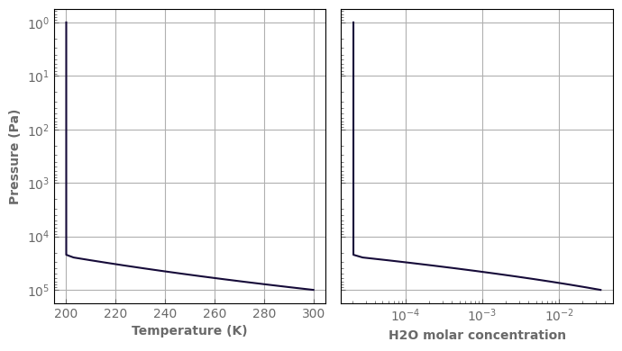
Here is an example of an Earth with a moist troposphere near saturation.
Notice that for the concentrations, you can put either a single value or an array (or a mix), as long as the size of the array is the same as the size of the T-logP arrays.
[10]:
Nlay = 100  # Number of layers
Tsurf = 300.  # K => Surface temperature
Tstrat = 200.  # K => Temperature of the stratosphere
psurf = 1.e5  # Pa => Surface pressure
ptop = 1.e0  # Pa => Pressure at the model top
grav = 9.81  # m/s^2 => Surface gravity
rcp = 0.28  # dimless => R/cp #create the layer pressure grid
Rp = 1. * u.Rearth  # m => Planetary radius
albedo_surf = 0.2  # m => Surface albedo

logplay = np.linspace(np.log10(ptop), np.log10(psurf), Nlay)
# design your adiabat
tlay = Tsurf * (10 ** logplay / psurf) ** rcp
tlay = np.where(tlay < Tstrat, Tstrat, tlay)

# create your composition. Here, only water is variable and follows saturation.
h2o_thermo_params = {
        'Latent_heat_vaporization': 2.486e6, 'cp_vap': 4.228e3, 'Mvap': 18.e-3,
        'T_ref'                   : 273., 'Psat_ref': 612.}
h2o = xk.Condensing_species(**h2o_thermo_params)
psat_h2o = h2o.Psat(tlay)
x_h2o = psat_h2o / (psat_h2o + 10 ** logplay)
for i in range(len(x_h2o) - 2, -1, -1):
    if x_h2o[i + 1] < x_h2o[i]:
        x_h2o[i] = x_h2o[i + 1]

composition = {'CO2': 4.e-4, 'H2O': x_h2o, 'N2': 'background'}

#Loads the atmosphere and computes some intermediate things
atm_earth = xk.Atm(logplay=logplay, tlay=tlay, grav=grav,
                   Rp=Rp, rcp=rcp,
                   albedo_surf=albedo_surf,
                   composition=composition,
                   k_database=k_db, cia_database=cia_db,
                   rayleigh=True)
[11]:
fig, axs = plt.subplots(1, 2, sharey=True, figsize=(7, 4))
atm_earth.plot_T_profile(axs[0], yscale='log')
axs[1].plot(x_h2o, atm_earth.play)
axs[1].set_xscale('log')
axs[1].set_xlabel('H2O molar concentration')
fig.tight_layout()
Changing attributes of an atmosphere
In an atmosphere, many attributes are interrelated and cannot be changed separately. Changing the pressures, for example, will change the mass of the atmosphere, the altitudes, etc.
So, if you want to change some attributes of the instance you are working with after it has been created, it is recommended to use the methods made for that. Here is a non-exhaustive list: set_logPT_profile, set_T_profile(), set_grav(), set_gas(), set_Mgas(), set_rcp(), set_Rp(), set_Rstar(), set_k_database(), set_cia_database(), set_spectral_range(), set_incoming_stellar_flux(), set_internal_flux(), set_surface_albedo(),
set_rayleigh().
See the API reference for completeness.
Optional attributes
At the initialisation, a Mgas can be specified to force a molar mass whatever the composition.
With wn_range or wl_range one can limit the wavenumber/wavelength range of future computations.
flux_top_dw (w/m^2) allows you to specify the stellar flux impinging on the top of the atmosphere. If you do not specify anything else, the spectral energy distribution will be the one of a blackbody at T=5778K. This temperature can be changed by using the Tstar keyword at the same time. Alternatively, one can provide a Spectrum object with the keyword stellar_spectrum. This spectrum must be in units of power per wavenumber. The actual units are irrelevant as this spectrum will
be renormalized with the value of flux_top_dw provided.
Transmission spectroscopy
To compute the transmission spectrum for your atmosphere, you can use the following method. Among the available options, there is rayleigh, Rstar,
[12]:
Rs = 1. * u.Rsun  # m => Radius of the star to compute the transit depth

spec = atm_hotjup.transmission_spectrum(Rstar=Rs, rayleigh=True)
Important
The result of transmission_spectrum() is a Spectrum
object onto which some methods can be used like
plotting, binning, and some algebraic operations.
[13]:
fig, ax = plt.subplots(1, 1, sharex=True, sharey=True)
spec.plot_spectrum(ax, xscale='log', label='Native corr-k resolution')
# bin_down_cp makes a deep copy before binning so that we keep the initial Spectrum instance
spec.bin_down_cp(xk.wavenumber_grid_R(400., 30000., 200)).plot_spectrum(ax, xscale='log', label=r'$R=200$')
spec.bin_down_cp(xk.wavenumber_grid_R(400., 30000., 30)).plot_spectrum(ax, xscale='log', label=r'$R=30$')
ax.set_ylabel('Depth')
ax.legend()
fig.tight_layout()
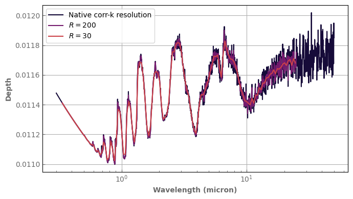
Notice that the stellar radius is now an attribute of the Atm instance and does not have to be repeated.
[14]:
assert atm_hotjup.Rstar == Rs.to_value(u.m)
Rayleigh scattering can be turned off for any given computation with the rayleigh=False keyword. However, if you want to turn it on/off permanently for the current instance, you can use atm_hotjup.set_rayleigh(rayleigh=True/False).
[15]:
spec_wo_rayleigh = atm_hotjup.transmission_spectrum(rayleigh=False)

fig, ax = plt.subplots(1, 1, sharex=True, sharey=True)
spec_wo_rayleigh.plot_spectrum(ax, xscale='log',label='w/o rayleigh')
spec.plot_spectrum(ax, xscale='log', linestyle='dotted',label='w rayleigh')
ax.set_ylabel('Depth')
fig.legend()
fig.tight_layout()

Emission spectroscopy
Exo_k enables several modes to compute the emission of a planet:
Atm.emission_spectrum(mu0=, **kwargs): Simple computation using Schwarzschild’s equation with mu0 as the cosine of the observer zenith angle. This mode cannot handle scattering. The output is given as a flux assuming a constant hemispheric intensity, but it can be used to compute the specific intensity at various angles by changing mu0.Atm.emission_spectrum(mu_quad_order=, **kwargs): This mode computes the specific intensity atmu_quad_orderangles and integrates it to yield the flux. Exact in the non-scattering limit. Cannot handle scattering.Atm.emission_spectrum_2stream(**kwargs): This mode computes the upward and downward fluxes using the constant hemispheric mean two-stream approximation of Toon et al. (1989). This mode can handle scattering and provides fluxes at all the layer interfaces (levels), so that radiative heating rates can be computed. In this case, a stellar flux must be specified.
As expected, in a non-scattering medium and with a zero surface albedo, Atm.emission_spectrum and Atm.emission_spectrum_2stream provide the same top of atmosphere outgoing flux almost down to machine precision. The second will be longer as it computes downward fluxes as well.
Computing top of atmosphere fluxes
[16]:
TOA_flux = atm_mars.emission_spectrum_2stream(
        wl_range=[0.1, 150.0],  #can reduce the wavelength range of the computation to save time
        #rayleigh=True, # whether rayleigh scattering is locally accounted for (even for thermal emission)
        )

Surf_blackbody = atm_mars.surf_bb()
TOA_blackbody = atm_mars.top_bb()
#print("Forward model duration:")
#%timeit -n 2 -r 2 atm_mars.emission_spectrum(integral=True, wl_range=[0.1,150.0])
#%timeit -n 2 -r 2 atm_mars.emission_spectrum_2stream(integral=True, wl_range=[0.1,150.0])
Important
The result of emission_spectrum() is a Spectrum
object onto which some methods can be used like:
computing the total flux, plotting, binning, and some algebraic operations
(subtract of divide spectra).
[17]:
print("Top of atmosphere flux:", TOA_flux.total, 'W/m^2')
print("Black body at Tsurf over the computed nu range is:", Surf_blackbody.total, 'W/m^2')
print('(sigma*Tsurf**4 is:', xk.SIG_SB * atm_mars.tlay[-1] ** 4, 'W/m^2)')
Top of atmosphere flux: 113.29278965856365 W/m^2
Black body at Tsurf over the computed nu range is: 123.8263545887508 W/m^2
(sigma*Tsurf**4 is: 132.8317491952 W/m^2)
[18]:
fig, axs = plt.subplots(1, 2, sharey=False, figsize=(8, 4))
Surf_blackbody.plot_spectrum(axs[0], label='Blackbody ($T_{surf}$)', linestyle='dotted')
TOA_blackbody.plot_spectrum(axs[0], label='Blackbody ($T_{strat}$)')
TOA_flux.plot_spectrum(axs[0], label='OLR')
Surf_blackbody.plot_spectrum(axs[1], per_wavenumber=False, label='Blackbody ($T_{surf}$)', linestyle='dotted')
TOA_blackbody.plot_spectrum(axs[1], per_wavenumber=False, label='Blackbody ($T_{strat}$)')
TOA_flux.plot_spectrum(axs[1], per_wavenumber=False, label='OLR')

axs[0].set_ylabel(r'Flux ($W/m^2/cm^{-1}$)')
axs[1].set_ylabel(r'Flux ($W/m^2/\mu m$)')
axs[1].set_xscale('log')
for ax in axs:
    ax.legend()
fig.tight_layout()
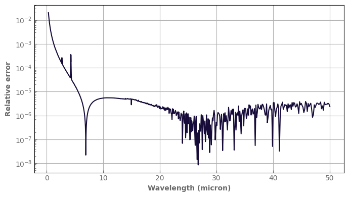
By default, the source function is integrated inside each bin. The user can specify integral=False to evaluate the Planck function at the center of the bins only. It is a little faster, but inaccurate for large bins. It can be used when using moderate to high-resolution radiative data.
Let’s see the error we would make with this mode (here at a resolution of 300) using algebraic operations on our spectra.
[19]:
TOA_flux_no_integral = atm_mars.emission_spectrum_2stream(
        integral=False,
        wl_range=[0.1, 150.0],  #can reduce the wavelength range of the computation to save time
        rayleigh=True,  # whether rayleigh scattering is accounted for (even for thermal emission)
        )
rel_error = ((TOA_flux_no_integral - TOA_flux) / TOA_flux).abs()  # .abs() to have the absolute value

fig, ax = plt.subplots(1, 1)
rel_error.plot_spectrum(ax, yscale='log')

ax.set_ylabel('Relative error')
fig.tight_layout()

Turning CIAs on and off
[20]:
# Computes emission flux for the two cases

atm_earth.set_cia_database(None)  # remove CIAs
TOA_flux_nocia = atm_earth.emission_spectrum()

atm_earth.set_cia_database(cia_db)  # reset CIAs
TOA_flux_cia = atm_earth.emission_spectrum_2stream()

Surf_blackbody = atm_earth.surf_bb()
TOA_blackbody = atm_earth.top_bb()

assert TOA_flux_cia.total < TOA_flux_nocia.total

print("Top of atmosphere flux:")
print("With CIAs   :", TOA_flux_cia.total, 'W/m^2')
print("Without CIAs:", TOA_flux_nocia.total, 'W/m^2')
print("we can see the reduced emission with CIAs")
Top of atmosphere flux:
With CIAs   : 260.76473363882496 W/m^2
Without CIAs: 291.0895104859162 W/m^2
we can see the reduced emission with CIAs
[21]:
fig, axs = plt.subplots(1, 2, sharey=False, figsize=(8, 4))
Surf_blackbody.plot_spectrum(axs[0], label='Blackbody ($T_{surf}$)')
TOA_blackbody.plot_spectrum(axs[0], label='Blackbody ($T_{strat}$)')
TOA_flux_nocia.plot_spectrum(axs[0], label=r'OLR w/o CIA')
TOA_flux_cia.plot_spectrum(axs[0], label=r'OLR w/ CIA')

Surf_blackbody.plot_spectrum(axs[1], per_wavenumber=False, label='Blackbody ($T_{surf}$)')
TOA_blackbody.plot_spectrum(axs[1], per_wavenumber=False, label='Blackbody ($T_{strat}$)')
TOA_flux_nocia.plot_spectrum(axs[1], per_wavenumber=False, label=r'OLR w/o CIA')
TOA_flux_cia.plot_spectrum(axs[1], per_wavenumber=False, label=r'OLR w/ CIA')

axs[0].set_ylabel(r'Flux ($W/m^2/cm^{-1}$)')
axs[1].set_ylabel(r'Flux ($W/m^2/\mu m$)')
axs[1].set_xscale('log')
for ax in axs:
    ax.legend()
fig.tight_layout()

Contribution Function
Once an emission spectrum has been computed, one can use the contribution_function() method to compute the spectral contribution function of each layer of the atmosphere. The result is an array of size (Number of radiative layers (Nlay-1), Number of wavenumber bins) that give the contribution function in the bin in W/m2/str/cm-1.
To integrate over a wavenumber band, one must multiply by the bin width before adding the values.
In the example below, one can see that in the 15 micron band of CO2, Earth’s atmosphere emission mostly comes from the lower stratosphere whereas the lower troposphere and surface contribute much more in the 10 micron radiative window.
[22]:
contribution_function = atm_earth.contribution_function()
fig, ax = plt.subplots(1, 1, sharey=False, figsize=(3, 4))
#for contrib in contribution_function.T:
#    ax.plot(contrib)
ax.plot(contribution_function[:, k_db['CO2'].wlindex(15.)], atm_earth.plev[1:-1], label=r'15 $\mu$m (CO$_2$ band)')
ax.plot(contribution_function[:, k_db['CO2'].wlindex(20.)], atm_earth.plev[1:-1], label=r'10 $\mu$m', linestyle='--')
ax.invert_yaxis()
ax.set_yscale('log')
ax.set_xlabel(r'Contribution Function (W/m$^2$/str/cm$^{-1}$)')
ax.set_ylabel(r'Pressure (Pa)')
ax.legend()
fig.tight_layout()

[23]:
origin = 'upper'
delta = 0.025

x = k_db.wls
y = atm_earth.play[1:]
X, Y = np.meshgrid(x, y)
Z = atm_earth.exp_minus_tau()

nr, nc = Z.shape

plt.rc('axes', grid=False)
fig, ax = plt.subplots(constrained_layout=True)
ax.invert_yaxis()
ax.set_xscale('log')
ax.set_yscale('log')
ax.set_xlim(left=0.3, right=20.)
CS = ax.contourf(X, Y, Z, 10, cmap=plt.cm.bone, origin=origin)
ax.set_title('Atm. Transmittance')
ax.set_xlabel('Wavelength (mu)')
ax.set_ylabel('Log(Pressure/Pa)')
# Make a colorbar for the ContourSet returned by the contourf call.
cbar = fig.colorbar(CS)
cbar.ax.set_ylabel('Exp(-tau)')
plt.rc('axes', grid=True)
# Add the contour line levels to the colorbar

Adding reflected light
To account for reflected light from the star, one just needs to specify the stellar flux impinging on the planet’s top-of-atmosphere (TOA) as well as the spectral energy density of the star.
To do this, there are two different modes to specify impinging stellar flux. The first one is where you set the temperature of a blackbody and the second one is where you specify the spectrum used.
Moreover, we also provide two modes to treat the stellar flux. The default one sets this flux as a boundary condition for the downwelling diffuse flux at the top and lets the solver treat it. The second one sets this flux as a source term, the flux is described as collimated. The contribution from the collimated flux is computed for each level and given to the solver. This allows us to take into account the angle of the collimated flux, whereas in the first case, the solver diffuses stellar contribution along the line of sight.
Important
Whatever the method used to describe the incoming flux, flux_top_dw is always the value of the bolometric incoming flux, i.e. the flux received at the top of the column per unit surface of the colum (so the stellar flux times the cosine of the zenith angle). Even when a stellar zenith angle is provided (e.g. for the collimated flux option), the code will NOT multiply by the cosine of the zenith angle internally.
Using a stellar blackbody
For this mode, you just need to specify the bolometric stellar flux at the TOA (in W/m^2) with the flux_top_dw keyword, and the stellar temperature with the Tstar keyword at initialization (or using Atm.set_incoming_stellar_flux()).
[24]:
Nlay = 50  # Number of layers
Tsurf = 200.  # K => Surface temperature
Tstrat = 100.  # K => Temperature of the stratosphere
psurf = 640.  # Pa => Surface pressure
ptop = 1.e0  # Pa => Pressure at the model top
grav = 3.4  # m/s^2 => Surface gravity
rcp = 0.28  # dimless => R/cp
Rp = None  # m => Planetary radius
albedo_surf = 0.2  # m => Surface albedo
wn_albedo_cutoff = 5000.

Tstar = 5570.  # K => Stellar blackbody temperature
flux_top_dw = 120.  # W/m^2 => stellar flux at the TOA.

composition = {'CO2': 'background', 'H2O': 1.e-6}
# Volume molar concentrations of the various species
# One gas can be set to `background`.
# It's volume mixing ratio will be automatically computed to fill the atmosphere.

atm_mars = xk.Atm(psurf=psurf, ptop=ptop,
                  Tsurf=Tsurf, Tstrat=Tstrat,
                  grav=grav, rcp=rcp, Rp=Rp,
                  albedo_surf=albedo_surf,
                  wn_albedo_cutoff=wn_albedo_cutoff,
                  composition=composition, Nlay=Nlay,
                  k_database=k_db, cia_database=cia_db,
                  rayleigh=True,
                  flux_top_dw=flux_top_dw, Tstar=Tstar, # Set the arguments for the stellar flux
                  )
[25]:
TOA_flux = atm_mars.emission_spectrum_2stream(source=False)

Surf_blackbody = atm_mars.surf_bb()
TOA_blackbody = atm_mars.top_bb()
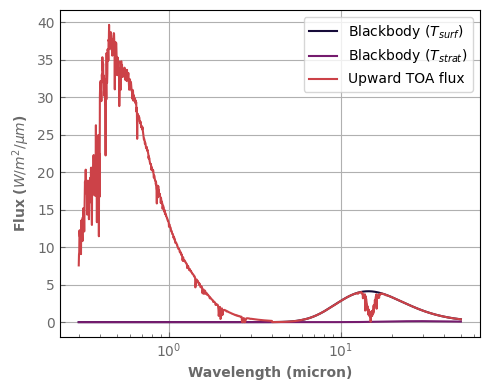
[26]:
fig, ax = plt.subplots(1, 1, figsize=(5, 4))
Surf_blackbody.plot_spectrum(ax, per_wavenumber=False, label='Blackbody ($T_{surf}$)')
TOA_blackbody.plot_spectrum(ax, per_wavenumber=False, label='Blackbody ($T_{strat}$)')
TOA_flux.plot_spectrum(ax, per_wavenumber=False, label='Upward TOA flux')

ax.set_ylabel(r'Flux ($W/m^2/\mu m$)')
ax.set_xscale('log')
ax.legend()
fig.tight_layout()

Important
By default, the surface albedo becomes 0. above 2 microns (5000 cm^-1). You can change that with the wn_albedo_cutoff argument at initialization.
Using an input stellar spectrum
We first have to load a stellar spectrum in a Spectrum object.
For this, we can provide an ascii file with two columns, the first one being the spectral axis, and the second one the radiance in flux per spectral unit.
The code assumes that the spectral quantity (wavelength or wavenumber) and units used are the same for both columns (for example a flux in W/micron if the spectral unit is microns. Fluxes in number of photons are not supported).
The precise units for the flux have no importance as the spectrum will be renormalized when input into the model. So any multiplicative factor will be lost.
[27]:
stellar_spectrum = xk.Spectrum(filename='../data/stellar_spectra/solar_spectrum.dat',
                               spectral_radiance=True, input_spectral_unit='nm')

fig, ax = plt.subplots(1, 1, figsize=(5, 4))
stellar_spectrum.plot_spectrum(ax)
ax.set_ylabel(r'Flux ($W/m^2/cm^{-1}$)')
ax.set_xscale('log')
fig.tight_layout()
[28]:
Tstar = None  # K => Stellar blackbody temperature

atm_mars = xk.Atm(psurf=psurf, ptop=ptop,
                  Tsurf=Tsurf, Tstrat=Tstrat,
                  grav=grav, rcp=rcp, Rp=Rp,
                  albedo_surf=albedo_surf,
                  wn_albedo_cutoff=wn_albedo_cutoff,
                  composition=composition, Nlay=Nlay,
                  k_database=k_db, cia_database=cia_db,
                  rayleigh=True,
                  flux_top_dw=flux_top_dw,
                  Tstar=Tstar,
                  stellar_spectrum=stellar_spectrum,
                  )
[29]:
TOA_flux = atm_mars.emission_spectrum_2stream(source=False)

Surf_blackbody = atm_mars.surf_bb()
TOA_blackbody = atm_mars.top_bb()
[30]:
fig, ax = plt.subplots(1, 1, figsize=(5, 4))
Surf_blackbody.plot_spectrum(ax, per_wavenumber=False, label='Blackbody ($T_{surf}$)')
TOA_blackbody.plot_spectrum(ax, per_wavenumber=False, label='Blackbody ($T_{strat}$)')
TOA_flux.plot_spectrum(ax, per_wavenumber=False, label='Upward TOA flux')

ax.set_ylabel(r'Flux ($W/m^2/\mu m$)')
ax.set_xscale('log')
ax.legend()
fig.tight_layout()

Treating the stellar flux as a collimated flux
By default, the stellar flux is treated as a diffusive flux arriving at the top of the atmosphere (stellar_mode='diffusive'). You can set stellar_mode='collimated' to treat it as a collimated ray of light whose (cosine) zenith angle is mu_star.
The first mode sets the received flux as a boundary condition, the solver transports it along an effective direction along with all the other photons in a 2 stream approximation (with a cosine of the effective angle being mu0). The second mode allows to transport it along a given direction independent of the observer (mu_star).
Important
As for the diffusive mode, flux_top_dw is still the bolometric incoming flux, i.e. the flux received at the top of the column (so the stellar flux times mu_star). The code will NOT multiply by the cosine of the zenith angle internally.
The following example demonstrates the use of the stellar_mode='collimated'. One can see that the reflected flux is the same with the ‘diffusive and ‘collimated’ approach as long as mu_star is equal to the effective angle mu0 which is 0.5 by default. However, we recover the fact that the albedo insreases when the star is closer to the horizon.
Recall that:
atm_mars = xk.Atm(...,
                  flux_top_dw=flux_top_dw,
                  Tstar=Tstar, # <- we choose to use a blackbody
                  ...)
[31]:
common_kwargs = {
        'mu0': 0.5,  # using an effective direction of 60 degrees for the 2 stream calculation
        'wl_range':[0.3,2.],
        }
atm_earth.set_incoming_stellar_flux(flux_top_dw=flux_top_dw, stellar_spectrum=stellar_spectrum)
TOA_flux_diffusive = atm_earth.emission_spectrum_2stream(**common_kwargs)

# this case shows that the results are equal when using mu_star=mu0
TOA_flux_collimated = atm_earth.emission_spectrum_2stream(stellar_mode='collimated',
                                                         mu_star=0.5,  # Set the mode and angle
                                                         **common_kwargs)

# this case shows that much more visible light is absorbed when the star is low on the horizon
TOA_flux_collimated_smallangle = atm_earth.emission_spectrum_2stream(stellar_mode='collimated',
                                                         mu_star=.01,  # Set the mode and angle
                                                         **common_kwargs)

# This attribute yields the spectrum of the incoming light at the top of atmosphere to compute the albedo
spectral_incoming_flux = atm_earth.spectral_incoming_flux
[32]:
fig, ax = plt.subplots(1, 1, figsize=(6, 4), squeeze=True)
ax = [ax]
(TOA_flux_collimated_smallangle/spectral_incoming_flux).plot_spectrum(ax[0], label=r'Collimated ($\mu_{star}=0.01$)', linestyle='dashed')
(TOA_flux_collimated/spectral_incoming_flux).plot_spectrum(ax[0], label=r'Collimated ($\mu_{star}=0.5$)')
(TOA_flux_diffusive/spectral_incoming_flux).plot_spectrum(ax[0], label=r'Diffusive ($\mu_0=0.5$)', linestyle='dotted')

ax[0].set_ylabel(r'Albedo')
ax[0].set_title(r'Reflected light')
ax[0].set_xscale('log')
ax[0].legend()


fig.tight_layout()

Heating rates
A by-product of the computation of the various fluxes in the atmosphere is that we know how much radiative energy is deposited and reradiated by each atmospheric layer, i.e. the heating rates.
They can be computed as follows:
[33]:
heat_rates, net_fluxes = atm_mars.heating_rate()
# Heat_Rate are the heating rates in each layer in W/kg (from the top-down)
# net_fluxes are the net bolometric fluxes (positive upward) in W/m^2 at the top of each layer.
[34]:
fig, axs = plt.subplots(1, 3, sharey=True)
axs[0].set_yscale('log')
axs[0].plot(heat_rates, atm_mars.play, label='Solar Heating')
axs[1].plot(net_fluxes, atm_mars.play, label='Net solar flux')
axs[2].plot(atm_mars.tlay, atm_mars.play)
axs[0].set_xlabel('Heating Rate (W/kg)')
axs[1].set_xlabel(r'Flux (W/m$^2$)')
axs[2].set_xlabel('Temperature (K)')
axs[0].set_ylabel('Pressure (Pa)')
axs[0].invert_yaxis()
fig.subplots_adjust(hspace=0, wspace=0)
fig.tight_layout()

In our example above, one can easily see from the left panel that the atmosphere is not in radiative equilibrium locally: * the surface receives more energy than it emits, whereas the troposphere below the 1mbar level wants to cool, which should drive convection.
The heating rates in the stratosphere are positive which means that it is too cold and wants to warm.
Finally, it can be seen in the middle panel that the atmosphere is not in a global radiative balance either, a negative net flux meaning that the atmosphere receives more light from its star than it can emit.
Bringing the atmosphere back to equilibrium will be the topic of the next section. In the meantime, to have a more complete diagnostic, it is possible to compute the heating rates and fluxes separately for the stellar and self-emission contributions.
[35]:
Fup_emis, Fdw_emis, Fnet_emis, H_emis, \
    Fup_stel, Fdw_stel, Fnet_stel, H_stel = atm_mars.bolometric_fluxes_2band()
[36]:
fig, axs = plt.subplots(1, 3, sharey=True)
axs[0].set_yscale('log')
axs[0].plot(H_stel, atm_mars.play, label='Stellar')
axs[0].plot(H_emis, atm_mars.play, label='Emis')
axs[1].plot(Fdw_stel, atm_mars.play, label='Stellar down')
axs[1].plot(Fup_stel, atm_mars.play, label='Stellar up')
axs[1].plot(Fdw_emis, atm_mars.play, label='Emis down')
axs[1].plot(Fup_emis, atm_mars.play, label='Emis up')
axs[2].plot(Fnet_stel, atm_mars.play, label='Stellar net')
axs[2].plot(Fnet_emis, atm_mars.play, label='Emis net')
axs[0].set_xlabel('Heating Rate (W/kg)')
axs[1].set_xlabel(r'Flux (W/m$^2$)')
axs[2].set_xlabel(r'Flux (W/m$^2$)')
axs[0].set_ylabel('Pressure (Pa)')
axs[0].legend(loc='upper left', fontsize='small')
axs[1].legend(loc='best', fontsize='small')
axs[2].legend(loc='best', fontsize='small')
axs[0].set_xlim((-0.3, 0.3))
axs[0].invert_yaxis()
fig.tight_layout()

Modeling atmospheric evolution with Atm_evolution
Now that we know how to model the radiative transfer (and heating rates) for a given atmospheric structure and composition, it is easy to predict how it evolves in time.
In Exo_k, this is handled by the Atm_evolution class that we present in this section.
Tailoring radiative data
During an evolution, the radiative transfer may be called hundreds of thousands of times. Furthermore, we do not need a high resolution to compute precise heating rates.
Therefore, to gain computation time, we will reduce the resolution of our Ktables. We will also make sure to extend its spectral range to capture the whole planetary and stellar spectral range.
For the demonstration, we will use a really coarse resolution, but one should of course test how the spectral grid affects their results to choose an appropriate setup.
[37]:
Res = 8.  #.4 # Using very low resolution for sake of speed
wn_grid_LR = xk.wavenumber_grid_R(100., 35000., Res)
print(wn_grid_LR)

k_db = xk.Kdatabase(['CO2', 'H2O'], 'R300_0.3-50mu.ktable.SI')
k_db_LR = k_db.bin_down_cp(wnedges=wn_grid_LR, remove_zeros=True)

cia_db_LR = xk.CIAdatabase(molecules=['N2', 'H2O', 'H2', 'He'], mks=True)
cia_db_LR.sample(k_db_LR.wns)
[  100.           113.31484531   128.40254167   145.49914146
   164.87212707   186.82459574   211.70000166   239.8875294
   271.82818285   308.02168489   349.03429575   395.50767229
   448.16890703   507.84190372   575.4602676    652.08191203
   738.90560989   837.28974881   948.77358364  1075.10131861
  1218.24939607  1380.45741861  1564.26318842  1772.54241215
  2008.55369232  2275.98950935  2579.03399172  2922.42837812
  3311.54519587  3752.47231596  4252.10820001  4818.26982911
  5459.81500331  6186.78092504  7010.54123467  7943.98395523
  9001.71313005 10200.27730827 11558.42845272 13097.41532108
 14841.31591026 16817.41416518 19056.62684586 21593.98723106
 24469.19322642 27727.22845231 31419.06602857 35000.        ]
[38]:
fig, ax = plt.subplots(1, 1, figsize=(5, 4))
k_db['H2O'].plot_spectrum(ax, p=1., t=300., g=1., xscale='log', yscale='log')
k_db_LR['H2O'].plot_spectrum(ax, p=1., t=300., g=1., xscale='log', yscale='log')
ax.set_ylim((1.e-34, 1.e-20))
ax.set_xlim((0.4, 10.))
fig.tight_layout()

Initializing an atmospheric evolution
Except for a few exceptions that we will discuss in more detail, the initialization of an Atm_evolution instance requires the same arguments as the initialization of an Atm object. The initial temperature profile can be specified exactly the same way, with the same options.
The most notable exceptions are: * bg_vmr: The molar concentrations (sometimes called the volume mixing ratios) of the various molecules constituting the background gas. This replaces the composition argument in a standard Atm object, but takes the same type of input. The reason for this change of name will be more evident in the next sections when we include active tracers (such as condensible species). bg_vmr can receive a dictionary of arrays if one wants to model an
atmosphere with a fixed (but not uniform) distribution of gases. Variable compositions will be treated later. * cp: Specific heat capacity of the gas at constant pressure (J/kg/K), that is needed to compute a temporal evolution. If it is not given, the code will try to compute it for some known molecules at a standard temperature. * M_bg: molar mass of the background gas (kg/mol; optional). It is possible to use a fixed molar mass of the background gas instead of the one computed from
the bg_vmr.
[39]:
Nlay = 50  # Number of layers
Tsurf = 200.  # K => Surface temperature
Tstrat = 100.  # K => Temperature of the stratosphere
psurf = 640.  # Pa => Surface pressure
ptop = 1.e0  # Pa => Pressure at the model top
grav = 3.4  # m/s^2 => Surface gravity
rcp = 0.28  # dimless => R/cp
Rp = None  # m => Planetary radius
albedo_surf = 0.2  # m => Surface albedo
Tstar = 5570.  # K => Stellar blackbody temperature
flux_top_dw = 120.  # W/m^2 => stellar flux at the TOA.

composition = {'CO2': 'background', 'H2O': 1.e-6}
# Volume molar concentrations of the various species
# One gas can be set to `background`.
# It's volume mixing ratio will be automatically computed to fill the atmosphere.

evol_mars = xk.Atm_evolution(Nlay=Nlay, psurf=psurf, ptop=ptop,
                             Tsurf=Tsurf, Tstrat=Tstrat,
                             grav=grav, rcp=rcp, Rp=Rp,
                             albedo_surf=albedo_surf,
                             bg_vmr=composition,  # notice the change in argument name
                             k_database=k_db_LR, cia_database=cia_db_LR,
                             rayleigh=True,
                             flux_top_dw=flux_top_dw, Tstar=Tstar)
[40]:
t_ini = evol_mars.atm.tlay
p_ini = evol_mars.atm.play

fig, ax = plt.subplots(1, 1, figsize=(3, 4))
evol_mars.atm.plot_T_profile(ax, yscale='log')
fig.tight_layout()

Setting evolution options
Now, that we have an initial atmospheric structure, we must decide what processes we will take into account when modeling its evolution, along with some parameters.
Here is a (non-exhaustive) list of the (frequently evolving) available options: * rayleigh (bool, default: True) * convection (bool, default: False) * convective_transport (bool, default: True) * diffusion (bool, default: False) * condensation (bool, default: False) * rain (bool, default: False) * latent_heating (bool, default: True) * moist_convection (bool, default: False) * moist_inhibition (bool, default: False) * dTmax_use_kernel (float,
default: 10.): Maximum temperature difference above which the full radiative transfer is recomputed. A small value increases the computation time. Too large a value may result in numerical instabilities. (See the theoretical description of the evolution model). * acceleration_mode (int, default: 0): What kind of physical acceleration scheme do you want to use. 0 means no acceleration. 4 is the most aggressive.
These options can be set at initialization or changed at any time through the ``set_options`` method.
[41]:
evol_mars.set_options(convection=True, dTmax_use_kernel=0.,
                      flux_top_dw=130.,
                      internal_flux=10., )
The set_options method can also be used to change some attributes of the underlying atmosphere and/or radiative transfer, like the radiative data used, or whether one wants to include the CIA, the stellar spectrum, etc. As these changes entail the re-initialization of the underlying Atm instance, including the recomputation of the radiative kernel, it is more efficient to do all these changes in a single call to set_options or even to set them directly at the initialization of the
Atm_evolution object.
Computing a time evolution
To move the model forward in time, you just need to call the evolve(N_timestep=) method where N_timestep is the number of timesteps that you want to run.
The duration of those timesteps will be decided by the model to be the largest stable timestep. If the user wants to reduce the timestep, it can specify a timestep_factor which must be <=1. A larger timestep_factor usually (although not always) results in unstable evolutions.
You can call evolve() as many times as you want. It will always pick up just where you left off.
[42]:
def plot_evolution(model, figsize=(6, 6), write=False):
    """A small routine to make standard plots of the evolution.
    It returns the figure and axis objects.
    Customize at will.
    """
    time_evo = model.time_hist / xk.DAY
    if write:
        print('evol_time (days):', time_evo[-1])
        print('last timestep:', (time_evo[-1] - time_evo[-2]), 'day')
        print('Number of steps since last kernel computation:', model.N_last_ker)
    fig, axs = plt.subplots(2, 1, sharex=True, figsize=figsize)
    axs[0].plot(time_evo, model.Fnet_top, label='Top of Atmosphere')
    axs[0].plot(time_evo, np.ones_like(model.Fnet_top) * model.atm.internal_flux,
                label='internal flux')
    axs[1].plot(time_evo, model.tlay_hist[:, -1], label='internal flux')
    axs[0].set_ylabel(r'Net Flux')
    axs[1].set_ylabel(r'$T_{surf}$')
    axs[1].set_xlabel(r'Time (days)')
    axs[0].legend()
    fig.tight_layout()
    return fig, axs
[43]:
model = evol_mars
start = time.time()

model.evolve(N_timestep=100)  # where the magic happens

print('simulation time:', time.time() - start, 's')

fig, axs = plot_evolution(model, write=True)
simulation time: 4.396235466003418 s
evol_time (days): 5.910935579671086
last timestep: 0.046531101171867206 day
Number of steps since last kernel computation: 100

One can see that the surface is warming up as the Net TOA flux is smaller than the internal flux (in this case, smaller than 0.).
Plotting profiles
We can also show the profiles for the: * Heating rates: in attribute H_ave[process] where process is a string that can be one of ‘rad’ (radiation), ‘conv’ (dry convection), ‘cond’ (condensation), ‘madj’ (moist convection), ‘rain’ (rain evaporation), ‘tot’ (total). They are given in W/kg and can be converted in K/s by dividing by self.cp. * Net fluxes: in attribute Fnet[process] where process is as above. They are given at the top of each layer in W/m^2. * Temperature and
pressure through self.atm.tlay and self.atm.play
[44]:
def plot_profiles(model, fig=None, axs=None, tracers=False, rh=False, figsize=(7, 4),
                  processes=None, mol='H2O', label_suffix=''):
    """A small routine to make standard plots of the atmospheric profiles.
    It returns the figure and axis objects.
    Customize at will.
    """
    if (fig is None) and (axs is None):
        if tracers:
            fig_loc, axs_loc = plt.subplots(1, 4, sharey=True, figsize=figsize)
            if processes is None:
                processes = ['rad', 'conv', 'madj', 'cond', 'rain', 'tot']
        else:
            fig_loc, axs_loc = plt.subplots(1, 3, sharey=True, figsize=figsize)
            if processes is None:
                processes = ['rad', 'conv', 'tot']
    else:
        fig_loc, axs_loc = fig, axs
    for label in processes:
        axs_loc[0].plot(model.heating_rate(label) * xk.DAY / model.cp, model.atm.play, label=label + label_suffix)
        axs_loc[1].plot(model.net_flux(label), model.atm.play, label=label + label_suffix)
    axs_loc[2].plot(model.atm.tlay, model.atm.play, label='Final' + label_suffix)
    axs_loc[0].set_ylabel(r'Pressure')
    axs_loc[0].set_xlabel(r'Heating (K/day)')
    axs_loc[1].set_xlabel(r'Fluxes')
    axs_loc[2].set_xlabel(r'T(K)')
    if tracers:
        if rh:
            axs_loc[3].plot(model.tracers[mol] / model.qsat(mol), model.atm.play, label=mol + label_suffix)
            axs_loc[3].set_xlabel(r'RH')
        else:
            axs_loc[3].plot(model.tracers[mol], model.atm.play, label=mol + label_suffix)
            axs_loc[3].plot(model.qsat(mol), model.atm.play, label=r'$q_{sat}$' + label_suffix, linestyle='--')
            axs_loc[3].set_xlabel(r'q (kg/kg)')
            axs_loc[3].set_xscale('log')
    for ax in axs_loc:
        ax.legend(fontsize='small', loc='upper right')
        ax.set_yscale('log')
    if fig is None:
        axs_loc[0].invert_yaxis()
        fig_loc.tight_layout()
    return fig_loc, axs_loc
[45]:
fig, axs = plot_profiles(evol_mars)
axs[2].plot(t_ini, p_ini, label='Ini')
_ = axs[2].legend(fontsize='small', loc='upper right')

As anticipated, the stratosphere was too cold and is now getting warmer.
If evolve is called again, the evolution will resume from its last point so that you can iteratively reach equilibrium.
Acceleration
Using the radiative kernel
Most of the time, we are only concerned with the equilibrium state of the atmosphere. However, it can take lots of iterations to get there. The evolution model thus includes several ways of accelerating the computation.
The easiest of all is to allow the model to use a linear approximation of a past radiative transfer computation if the temperature profile has not changed by more than dTmax_use_kernel Kelvin.
This can be changed as follows.
[46]:
evol_mars.set_options(dTmax_use_kernel=10.)
[47]:
model = evol_mars
start = time.time()
model.evolve(N_timestep=1000)

print('simulation time:', time.time() - start, 's')
fig, axs = plot_evolution(model, write=True)
simulation time: 2.709832191467285 s
evol_time (days): 46.50686219784943
last timestep: 0.04646825410230093 day
Number of steps since last kernel computation: 148

Notice that the simulation ran for almost as much time as before, but we have simulated a period about ten times as long (10 times the number of iterations).
The price to pay is those sawtooth patterns that appear each time we compute the kernel because our linear approximation was not that good anymore. These however do not affect the final equilibrium state as long as the model converges.
If dTmax_use_kernel is too large, the model may not converge.
Other acceleration modes
To reach equilibrium even faster it is possible to use other acceleration modes. They are described in the ‘Principles of atmospheric modeling with Exo_k’ page. They can be activated through the acceleration_mode argument as follows.
The most efficient one to date is acceleration_mode = 4 which accelerates both convective and radiative zones. Use acceleration_mode = 3 if you only want to accelerate radiative zones.
In this case and when we are close to equilibrium, it might be even faster to force the recomputation of the kernel a few times during an evolution step. This can be done through the evolve(N_kernel = ) argument that specifies a maximum number of steps between two computations of the kernel.
To show how fast this is, let’s compute the equilibrium for a new stellar flux.
[48]:
evol_mars.set_options(flux_top_dw=200., dTmax_use_kernel=10., acceleration_mode=4)
[49]:
model = evol_mars
start = time.time()

model.evolve(N_timestep=40, N_kernel=10)

print('simulation time:', time.time() - start, 's')
fig, axs = plot_evolution(model, write=True)
simulation time: 3.738776922225952 s
evol_time (days): 1.4575971406255608
last timestep: 0.034215032617129104 day
Number of steps since last kernel computation: 6

In only 40 iterations, we are almost in thermal equilibrium!
Saving and loading an atmospheric model
An atmospheric model can be saved to disc using serialization with:
[50]:
evol_mars.write_pickle('evol_mars.pickle')
Now, one can immediately load it again. It will have all of its attributes and options saved so that one can directly see the current state as well as make it evolve again.
[51]:
evol_mars2 = xk.load_atm_evolution('evol_mars.pickle')
[52]:
model = evol_mars2
try:
    model.evolve(N_timestep=40, N_kernel=10)
    print('I have all I need to evolve again')
except:
    print('This Atm_evolution instance is not linked to any k_database')
    print('We will reset the radiative model before running again')
    model.set_options(k_database=k_db_LR, cia_database=cia_db_LR)
    model.evolve(N_timestep=40, N_kernel=10)
print('simulation time:', time.time() - start, 's')
fig, axs = plot_evolution(model, write=True)
I have all I need to evolve again
simulation time: 6.944481611251831 s
evol_time (days): 1.3682042833552686
last timestep: 0.034196145300838365 day
Number of steps since last kernel computation: 0

[53]:
fig, axs = plot_profiles(evol_mars2)
axs[2].plot(t_ini, p_ini, label='Ini')
_ = axs[2].legend(fontsize='small', loc='upper right')

However, when saving it this way, the model may take some space on disk as it saves along all the opacity databases.
If one wants to save only the current state and the options, it is possible to use the data_reduction_level=2 argument in write_pickle.
However, if one wants to make the atmosphere evolve again, they will need to reset the radiative model with the opacities as follows
[54]:
evol_mars.write_pickle('evol_mars_small.pickle', data_reduction_level=2)

evol_mars3 = xk.load_atm_evolution('evol_mars_small.pickle')
[55]:
model = evol_mars3
try:
    model.evolve(N_timestep=40, N_kernel=10)
    print('I have all I need to evolve again')
except:
    print('We will reset the radiative model before running again')
    model.set_options(k_database=k_db_LR, cia_database=cia_db_LR)
    model.evolve(N_timestep=40, N_kernel=10)
print('simulation time:', time.time() - start, 's')
fig, axs = plot_evolution(model, write=True)
This Atm_evolution instance is not linked to any k_database
Use self.set_options(k_database=, ...)
We will reset the radiative model before running again
simulation time: 10.785094738006592 s
evol_time (days): 1.3681862894211634
last timestep: 0.034196117180982144 day
Number of steps since last kernel computation: 0

Equilibrating an atmosphere
While you can run evolve as many times as you want to reach equilibrium, the library also includes an equilibrate method that directly runs evolve until thermal equilibrium is met.
This method uses the following arguments: * Fnet_tolerance (W/m^2): The model will be considered equilibrated when the net TOA flux (corrected for the internal flux) will remain between + and - Fnet_tolerance during a call to evolve. * N_iter_max: the maximum number of calls to evolve. * N_timestep_ini: The number of timesteps in the first call to evolve. The number of timesteps will then be doubled each time until it reaches N_timestep_max. * verbose: to show
steps and diagnostics. * Any keyword argument for evolve can be passed.
Some atmospheres have an intrinsic variability. Fnet_tolerance must be large enough to account for this variability.
After a call to equilibrate, only the diagnostics for the last call to evolve are available (e.g. heating rates, fluxes, etc.)
[56]:
Nlay = 50  # Number of layers
Tsurf = 200.  # K => Surface temperature
Tstrat = 100.  # K => Temperature of the stratosphere
psurf = 640.  # Pa => Surface pressure
ptop = 1.e0  # Pa => Pressure at the model top
grav = 3.4  # m/s^2 => Surface gravity
rcp = 0.28  # dimless => R/cp
Rp = None  # m => Planetary radius
albedo_surf = 0.2  # m => Surface albedo
Tstar = 5570.  # K => Stellar blackbody temperature
flux_top_dw = 120.  # W/m^2 => stellar flux at the TOA.

composition = {'CO2': 'background', 'H2O': 1.e-6}
# Volume molar concentrations of the various species
# One gas can be set to `background`.
# It's volume mixing ratio will be automatically computed to fill the atmosphere.

evol_mars = xk.Atm_evolution(Nlay=Nlay, psurf=psurf, ptop=ptop,
                             Tsurf=Tsurf, Tstrat=Tstrat,
                             grav=grav, rcp=rcp, Rp=Rp,
                             albedo_surf=albedo_surf,
                             bg_vmr=composition,  # notice the change in argument name
                             k_database=k_db_LR, cia_database=cia_db_LR,
                             rayleigh=True,
                             flux_top_dw=flux_top_dw, Tstar=Tstar,
                             convection=True,
                             )

evol_mars.equilibrate(Fnet_tolerance=0.1, verbose=True)
fig, axs = plot_evolution(evol_mars, write=True)
fig, axs = plot_profiles(evol_mars)
iter: 1, N_timestep: 100
Fnet mean: -2.07 W/m^2, (min:-13.8, max:-0.544)
timestep: 0.0531 d | 4.59e+03 s, total time: 0.0148 yr
iter: 2, N_timestep: 200
Fnet mean: -0.476 W/m^2, (min:-0.552, max:-0.405)
timestep: 0.0531 d | 4.58e+03 s, total time: 0.0291 yr
iter: 3, N_timestep: 400
Fnet mean: -0.28 W/m^2, (min:-0.434, max:-0.161)
timestep: 0.053 d | 4.58e+03 s, total time: 0.0581 yr
iter: 4, N_timestep: 800
Fnet mean: -0.0612 W/m^2, (min:-0.201, max:-0.0111)
timestep: 0.053 d | 4.58e+03 s, total time: 0.116 yr
iter: 5, N_timestep: 1600
Fnet mean: -0.00405 W/m^2, (min:-0.0632, max:-2.69e-05)
timestep: 0.053 d | 4.58e+03 s, total time: 0.232 yr
evol_time (days): 84.78923852512237
last timestep: 0.052972721761506136 day
Number of steps since last kernel computation: 1600


Tracers and condensing species
Putting tracers in your model
Now let’s try to model an Earth-like planet with some water vapor in the atmosphere.
The first step is to add one or more tracers (at least two if you want a condensing species) through the tracers argument. The input is a dictionary whose keys are the tracer names and the values are another dictionary containing the properties of the tracer. In particular, for a condensing species, you want to specify that it is a 'type':'vapor' and the name of the condensed tracer with 'condensed_form':'H2O_liq' (This tracer must also be added. However, it does not need any
specific property).
There are several ways to specify the initial values/surface sources for the various tracers, as will be shown below. For the moment, let’s just add a constant initial mass concentration (kg/kg of gas) profile through 'init_value': q_h2o.
As we want the code to be as generic as possible, we must now specify the thermodynamical properties of the condensing pairs we want to model through the condensing_species argument. There is an example of water vapor below.
Thanks to this mechanism, there is no limitation on the number of condensing species that one can add, as long as we know the thermodynamical properties.
Important
The name of the vapor tracer must be the same as the name of the condensing species. This is how the library links the two. Moreover, if you want the vapor to be radiatively active, the name must be the same as the one in the Kdatabase. For example, here, putting ‘H2O_vap’ in tracers and condensible species would work, but water vapor would have no effect on the radiative transfer.
[57]:
# a simple function to test water conservation
def water_content(model):
    idx_vap, idx_cond = model.condensing_pairs_idx[model.condensing_species_idx['H2O']]
    return np.sum(model.tracers.qarray[idx_vap] * model.atm.dmass) \
        + np.sum(model.tracers.qarray[idx_cond] * model.atm.dmass) \
        + model.tracers.qsurf[idx_cond]
[58]:
Nlay = 50  # Number of layers
Tsurf = 280.  # K => Surface temperature
Tstrat = 150.  # K => Temperature of the stratosphere
psurf = 1.e5  # Pa => Surface pressure
ptop = 10.e0  # Pa => Pressure at the model top
grav = 9.81  # m/s^2 => Surface gravity
rcp = 0.28  # dimless => R/cp
Rp = None  # m => Planetary radius
albedo_surf = 0.35  # m => Surface albedo
Tstar = 5570.  # K => Stellar blackbody temperature
flux_top_dw = 340.  # W/m^2 => stellar flux at the TOA.

composition = {'N2': 'background', 'CO2': 340.e-6}

qH2O = 0.0001  # kg/kg of gas

# the tracers dictionary contains the tracers with their names and attributes.
# Here we have two: one for water vapor and one for the condensed phase.
# !!! The vapor one needs to have the same name as in the k_database if
#      the user wants to include its radiative effect !!!
tracers = {
        'H2O'    : {
                'type'          : 'vapor',  # a 'vapor' type specifies that it can condense
                'condensed_form': 'H2O_liq',  # if 'type'='vapor' then we need to specify the condensed form
                'init_value'    : qH2O,  # optional, the initial specific concentration (in kg/kg of total gas)
                },
        'H2O_liq': {},  # The tracer for the condensed form does not need any attribute
        }

# The condensing_species dictionary captures the necessary thermodynamical
# constant to compute the saturation curves and latent heat.
# There needs to be as many condensing_species as there are tracers with a vapor type.
condensing_species = {
        'H2O': {
                'Latent_heat_vaporization': 2.086e6,  # Latent heat at ref temperature (J/kg)
                'cp_vap'                  : 4.228e3,  # Specific heat of the vapor (J/kg/K)
                'Mvap'                    : 18.e-3,  # Molar mass of the vapor
                'T_ref'                   : 273.,  # Reference temperature
                'Psat_ref'                : 612.,  # Saturation pressure at reference temperature
                }}

tracer_values = None  # Dict with arrays of values for the various tracers.
# It is not needed here as we start with a constant value
# as specified above

evol_earth = xk.Atm_evolution(Nlay=Nlay, psurf=psurf, ptop=ptop,
                              Tsurf=Tsurf, Tstrat=Tstrat,
                              grav=grav, rcp=rcp, Rp=Rp,
                              albedo_surf=albedo_surf,
                              bg_vmr=composition,  # notice the change in argument name
                              k_database=k_db_LR, cia_database=cia_db_LR,
                              rayleigh=True,
                              flux_top_dw=flux_top_dw, Tstar=Tstar,
                              tracers=tracers, condensing_species=condensing_species,
                              tracer_values=tracer_values)

initial_water = water_content(evol_earth)
print("water content = ", initial_water, "kg/m^2")
water content = 1.0192660550458716 kg/m^2
Tracer related options
When (condensing) tracers are added, there are several additional options you can set. In particular: * Know that convection=True will instantaneously mix all tracers in convective zones. * condensation=True will condense vapors to bring any layer as close as possible to saturation equilibrium. * moist_convection=True calls a moist-convection adjustment scheme. * The effect of mean molecular weight on both dry and moist convection can be turned on with moist_inhibition=True.
* rain=True collects all the condensates left in the atmosphere by the previous processes and carries them downward until they are either re-evaporated or they reach the surface. * diffusion=True applies turbulent diffusive mixing to the tracers using a constant eddy mixing coefficient that is specified using Kzz=value (in m^2/s). This diffusion has no effect on temperature.
[59]:
# The moist processes are turned off by default and need to be turned on
evol_earth.set_options(convection=True, condensation=True,
                       moist_convection=True, moist_inhibition=True,
                       diffusion=True, Kzz=1.e-2,  # in m^2/s
                       rain=True,
                       acceleration_mode=0,
                       )
[60]:
model = evol_earth
start = time.time()
model.evolve(N_timestep=4000, timestep_factor=.01)
print('simulation time:', time.time() - start, 's')
print("water content:", water_content(model), "kg/m^2")
print("relative water mass loss:", (water_content(model) - initial_water) / initial_water)
fig, axs = plot_evolution(model, write=True)
simulation time: 17.671141862869263 s
water content: 1.0192660550460435 kg/m^2
relative water mass loss: 1.6861399765171188e-13
evol_time (days): 112.79539782148508
last timestep: 0.030106359657892767 day
Number of steps since last kernel computation: 3041

[61]:
fig, axs = plot_profiles(evol_earth, tracers=True)

Specifying initial tracer profiles and tracer sources
For the moment, there are two ways to specify the initial tracer distribution: * As seen above, 'init_value' in the tracers dictionary initializes the tracer with a constant specific concentration profile. * A vertical profile of specific concentration can be provided through tracer_values={'name_of_tracer: array}. The array must have the right size and be ordered from the top down, just like the other arrays.
If nothing else is specified, the model will evolve assuming that there is no surface source for tracers.
Tracer sources at the bottom boundary can be modelled with two different approaches: * By putting 'q_deep': value as a property of a given vapor tracer in tracers, you force the specific concentration for this vapor to remain fixed at this value in the surface layer. This is particularly useful to model gaseous planets with no definite surface. * By putting 'surface_reservoir': value as a property of a given condensate tracer in tracers, you specify that there is a
reservoir containing value kg/m^2 of the condensed species at the surface. The atmosphere can freely condense/evaporate matter to and from this reservoir depending on the thermodynamical conditions. This is particularly useful for modeling a surface ocean.
Setting up an ocean
The only line that changes to put an ocean is 'H2O_liq':{'surface_reservoir': 1000.},. Here we limit it to 1m (1000. kg/m^2).
[62]:
tracers = {
        'H2O'    : {
                'type'          : 'vapor',  # a 'vapor' type specifies that it can condense
                'condensed_form': 'H2O_liq',  # if 'type'='vapor' then we need to specify the condensed form
                'init_value'    : 0.,  # we start without any atm vapor
                },
        'H2O_liq': {'surface_reservoir': 1000.},  # here we put a 1m deep ocean
        }

evol_earth = xk.Atm_evolution(Nlay=Nlay, psurf=psurf, ptop=ptop,
                              Tsurf=Tsurf, Tstrat=Tstrat,
                              grav=grav, rcp=rcp, Rp=Rp,
                              albedo_surf=albedo_surf,
                              bg_vmr=composition,  # notice the change in argument name
                              k_database=k_db_LR, cia_database=cia_db_LR,
                              rayleigh=True,
                              flux_top_dw=flux_top_dw, Tstar=Tstar,
                              tracers=tracers, condensing_species=condensing_species,
                              tracer_values=tracer_values,
                              # evolution options
                              convection=True, condensation=True,
                              moist_convection=True, moist_inhibition=True,
                              diffusion=True, Kzz=1.e-1,  # in m^2/s
                              rain=True,
                              acceleration_mode=0,
                              mass_redistribution=False)
initial_water = water_content(evol_earth)
print("water content = ", initial_water, "kg/m^2")
water content = 1000.0 kg/m^2
[63]:
model = evol_earth
start = time.time()
model.evolve(N_timestep=2000, N_kernel=1000, timestep_factor=0.9)
print('simulation time:', time.time() - start, 's')
print("water content:", water_content(model), "kg/m^2")
print("relative water mass loss:", (water_content(model) - initial_water) / initial_water)
fig, axs = plot_evolution(model, write=True)
fig, axs = plot_profiles(evol_earth, tracers=True)
simulation time: 2.584286689758301 s
water content: 999.9999999999557 kg/m^2
relative water mass loss: -4.433786671143025e-14
evol_time (days): 7062.02525012997
last timestep: 3.5267880443852846 day
Number of steps since last kernel computation: 956


Forcing surface concentration
Here, the important option is 'q_deep':1.e-3.
Of course, in this setup, the tracer mass is not conserved as we have an open system.
Also, in this setting, you better make sure that the tracer does not condense at the surface or the model will be unstable.
[64]:
tracers = {
        'H2O'    : {
                'type'          : 'vapor',  # a 'vapor' type specifies that it can condense
                'condensed_form': 'H2O_liq',  # if 'type'='vapor' then we need to specify the condensed form
                'init_value'    : 0.,  # optional, the initial specific concentration (in kg/kg of total gas)
                'q_deep'        : 1.e-3,
                },
        'H2O_liq': {},  # The tracer for the condensed form does not need any attribute
        }

evol_earth = xk.Atm_evolution(Nlay=Nlay, psurf=psurf, ptop=ptop,
                              Tsurf=Tsurf, Tstrat=Tstrat,
                              grav=grav, rcp=rcp, Rp=Rp,
                              albedo_surf=albedo_surf,
                              bg_vmr=composition,  # notice the change in argument name
                              k_database=k_db_LR, cia_database=cia_db_LR,
                              rayleigh=True,
                              flux_top_dw=flux_top_dw, Tstar=Tstar,
                              tracers=tracers, condensing_species=condensing_species,
                              tracer_values=tracer_values,
                              # evolution options
                              convection=True, condensation=True,
                              moist_convection=True, moist_inhibition=True,
                              diffusion=True, Kzz=1.e1,  # in m^2/s
                              rain=True,
                              acceleration_mode=0,
                              mass_redistribution=False)
initial_water = water_content(evol_earth)
print("water content = ", initial_water, "kg/m^2")
water content = 0.0 kg/m^2
[65]:
model = evol_earth
start = time.time()
model.evolve(N_timestep=2000, N_kernel=1000, timestep_factor=0.01)
print('simulation time:', time.time() - start, 's')
print("water content:", water_content(model), "kg/m^2")
fig, axs = plot_evolution(model, write=True)
fig, axs = plot_profiles(evol_earth, tracers=True, rh=False)
simulation time: 2.029280424118042 s
water content: 5.002864739679519 kg/m^2
evol_time (days): 67.88826487171603
last timestep: 0.03324387089523384 day
Number of steps since last kernel computation: 889

