First steps with exo_k
Author: Jeremy Leconte (CNRS/LAB/Univ. Bordeaux)
The goal of exo_k is to provide a library to:
Interpolate efficiently and easily in correlated-k and cross section tables.
Convert easily correlated-k and cross section tables from one format to another (hdf5, LMDZ GCM, Exomol, Nemesis, PetitCode, TauREx, ExoREM, ARCIS, etc.).
Adapt precomputed correlated-k tables to your needs by changing:
the spectral and quadrature (g) grids,
the pressure/temperature grid.
Create tables for a mix of gases using tables for individual gases.
Create your own tables from high-resolution spectra.
Use your data in an integrated radiative transfer framework to simulate planetary atmospheres.
This first tutorial will show you how to deal with radiative data. The modeling of planetary atmospheres is detailed later on.
If you are reading this online, the executable notebook can be found there: https://forge.oasu.u-bordeaux.fr/jleconte/exo_k-public/-/blob/public/tutorials/tutorial-exo_k.ipynb
Initialization
exo_k.For this to work, you need to have installed the library by either typing
pip install exo_k
anywhere or
pip install -e .
at the root of exo_k directory (the location where you first saw this tutorial).
[1]:
import exo_k as xk
import numpy as np
import matplotlib.pyplot as plt
import astropy.units as u
import time,sys,os
[2]:
# Uncomment the line below if you want to enable interactive plots
#%matplotlib notebook
plt.rcParams["figure.figsize"] = (7,4)
from matplotlib import cycler
colors = cycler('color',[plt.cm.inferno(i) for i in np.linspace(0.1,1,5)])
plt.rc('axes', axisbelow=True, grid=True, labelcolor='dimgray', labelweight='bold', prop_cycle=colors)
plt.rc('grid', linestyle='solid')
plt.rc('xtick', direction='in', color='dimgray')
plt.rc('ytick', direction='in', color='dimgray')
plt.rc('lines', linewidth=1.5)
Important
Many global options can be changed after having imported the library using a syntax of the type
xk.Settings().method_name(args). Many examples will be provided along the way, but you
can have a look at exo_k.settings.Settings for all the possible options.
Documentation
The documentation in html form can be found at http://perso.astrophy.u-bordeaux.fr/~jleconte/exo_k-doc/index.html
It is searchable, and has a general index to find any function.
To access it through a python interface, just run the following line for any class, function, etc.:
[3]:
help(xk.Ktable().bin_down)
Help on method bin_down in module exo_k.ktable:

bin_down(wnedges=None, weights=None, ggrid=None, remove_zeros=False, num=300, use_rebin=False, write=0) method of exo_k.ktable.Ktable instance
    Method to bin down a kcoeff table to a new grid of wavenumbers (inplace).

    Parameters
    ----------
        wnedges: array, np.ndarray
            Edges of the new bins of wavenumbers (cm-1)
            onto which the kcoeff should be binned down.
            if you want Nwnew bin in the end, wnedges.size must be Nwnew+1
            wnedges[0] should be greater than self.wnedges[0] (JL20 not sure anymore)
            wnedges[-1] should be lower than self.wnedges[-1]
        weights: array, np.ndarray, optional
            Desired weights for the resulting Ktable.
        ggrid: array, np.ndarray, optional
            Desired g-points for the resulting Ktable.
            Must be consistent with provided weights.
            If not given, they are taken at the midpoints of the array
            given by the cumulative sum of the weights
Dealing with Ktable() objects
Loading and saving a Ktable() object
For this tutorial to work, you should launch this notebook from a base_directory that contains a data/corrk/ directory where your correlated k files are stored. You can download simple example data at https://forge.oasu.u-bordeaux.fr/amechineau/pytmosph3r-data/-/archive/minimal/pytmosph3r-data-minimal.zip. To download and move the data in the correct paths, you can uncomment the following cell:
[4]:
# ! wget https://forge.oasu.u-bordeaux.fr/amechineau/pytmosph3r-data/-/archive/minimal/pytmosph3r-data-minimal.zip
# ! unzip pytmosph3r-data-minimal.zip
# ! mkdir -p data
# ! mv pytmosph3r-data-minimal/* data/   # or if you already have data/, update it with: rsync -avz pytmosph3r-data-minimal/ data/
Many thanks to K. Chubb and the Exomol project for providing the data used in these examples.
[5]:
datapath = '../data/'
Loading a Ktable from a file
One of the main objects we will deal with is the Ktable() object. This contains a big matrix with k-coefficients for a species or a mix of species along with all the needed supporting information such as the Pressure, Temperature, wavenumber, and g grids onto which the k-coefficients have been computed.
To instantiate a Ktable() object from most currently supported formats, just run the following line. If you are specifying the file through the filename keyword, you have to give the full path to the file. The format should be recognized from the extension (see http://perso.astrophy.u-bordeaux.fr/~jleconte/exo_k-doc/units.html for supported formats).
See also
exo_k.ktable.Ktable() for details on arguments and options.
[6]:
h2o_ktab=xk.Ktable(filename=datapath + 'corrk/H2O_R300_0.3-50mu.ktable.TauREx.h5')
print(h2o_ktab)
        file         : ../data/corrk/H2O_R300_0.3-50mu.ktable.TauREx.h5
        molecule     : H2O
        p grid       : [1.00000000e-05 2.15443469e-05 4.64158883e-05 1.00000000e-04
 2.15443469e-04 4.64158883e-04 1.00000000e-03 2.15443469e-03
 4.64158883e-03 1.00000000e-02 2.15443469e-02 4.64158883e-02
 1.00000000e-01 2.15443469e-01 4.64158883e-01 1.00000000e+00
 2.15443469e+00 4.64158883e+00 1.00000000e+01 2.15443469e+01
 4.64158883e+01 1.00000000e+02]
        p unit       : bar
        t grid   (K) : [ 100.  200.  300.  400.  500.  600.  700.  800.  900. 1000. 1100. 1200.
 1300. 1400. 1500. 1600. 1700. 1800. 1900. 2000. 2200. 2400. 2600. 2800.
 3000. 3200. 3400.]
        wn grid      : [  199.90345491   200.56979976   201.23836576 ... 33057.12210094
 33167.31250795 33277.87021631]
        wn unit      : cm^-1
        kdata unit   : cm^2/molecule
        weights      : [0.008807   0.02030071 0.03133602 0.04163837 0.05096506 0.05909727
 0.06584432 0.07104805 0.07458649 0.07637669 0.07637669 0.07458649
 0.07104805 0.06584432 0.05909727 0.05096506 0.04163837 0.03133602
 0.02030071 0.008807  ]
        data oredered following p, t, wn, g
        shape        : [  22   27 1538   20]
Managing Units
Tracking units
Except for self-defining formats (such as hdf5), most formats handled by exo_k do not carry the information on units with them (Exo_transmit, HITRAN .cia, etc.).
However, previous experience has shown us that tracking units is essential to avoid errors and working with SI units is recommended when possible.
For this reason, the units for pressure, kdata, and wavenumbers are kept as attributes of any Ktable object. They can be seen by printing the object (as above). If the input format is self-defining (e.g. hdf5) the units are read in the file. For all the other formats, the units are assumed to always be the same and have been inferred from reading the codes using these formats and their documentation (see http://perso.astrophy.u-bordeaux.fr/~jleconte/exo_k-doc/units.html for some examples and a more general discussion).
Converting to new units
To control the unit we want to work with, we just need to specify what units we want with the p_unit and kdata_unit keywords.
These keywords accept string input with units recognized by the astropy.units library such as ‘Pa’, ‘mbar’, and ‘bar’ for pressure and e.g. ‘m^2/molecule’ and ‘cm^2/molecule’ for cross sections. Although ‘/molecule’ is not a unit recognized by astropy.units, it is automatically appended to the unit string provided by the user when necessary as a reminder that opacities per ‘moles’ or ‘kg’ are not supported.
To use SI units, just reload your ktable as shown below. Note that you can also force SI units to be used with the global option to be set once and for all.
xk.Settings().set_mks(True)
[7]:
h2o_ktab_SI=xk.Ktable(filename=datapath + 'corrk/H2O_R300_0.3-50mu.ktable.TauREx.h5',
                         kdata_unit='m^2', p_unit='Pa')
# or simply
xk.Settings().set_mks(True)
h2o_ktab_SI=xk.Ktable(filename=datapath + 'corrk/H2O_R300_0.3-50mu.ktable.TauREx.h5')
print(h2o_ktab_SI)
        file         : ../data/corrk/H2O_R300_0.3-50mu.ktable.TauREx.h5
        molecule     : H2O
        p grid       : [1.00000000e+00 2.15443469e+00 4.64158883e+00 1.00000000e+01
 2.15443469e+01 4.64158883e+01 1.00000000e+02 2.15443469e+02
 4.64158883e+02 1.00000000e+03 2.15443469e+03 4.64158883e+03
 1.00000000e+04 2.15443469e+04 4.64158883e+04 1.00000000e+05
 2.15443469e+05 4.64158883e+05 1.00000000e+06 2.15443469e+06
 4.64158883e+06 1.00000000e+07]
        p unit       : Pa
        t grid   (K) : [ 100.  200.  300.  400.  500.  600.  700.  800.  900. 1000. 1100. 1200.
 1300. 1400. 1500. 1600. 1700. 1800. 1900. 2000. 2200. 2400. 2600. 2800.
 3000. 3200. 3400.]
        wn grid      : [  199.90345491   200.56979976   201.23836576 ... 33057.12210094
 33167.31250795 33277.87021631]
        wn unit      : cm^-1
        kdata unit   : m^2/molecule
        weights      : [0.008807   0.02030071 0.03133602 0.04163837 0.05096506 0.05909727
 0.06584432 0.07104805 0.07458649 0.07637669 0.07637669 0.07458649
 0.07104805 0.06584432 0.05909727 0.05096506 0.04163837 0.03133602
 0.02030071 0.008807  ]
        data oredered following p, t, wn, g
        shape        : [  22   27 1538   20]
Now both the pressure unit and the pressure grid have changed!
Overriding default units in a file
If for some reason you know that the units used in a given input file are different from the default ones assumed for this format, you can always override the default units by explicitly stating what are the pressure (file_p_unit keyword) and k-coefficient (file_kdata_unit keyword) units.
Let’s say, for example, that you know the pressures in the above file where in fact given in mbar, you could specify it using
[8]:
xk.Ktable(filename=datapath + 'corrk/H2O_R300_0.3-50mu.ktable.TauREx.h5', file_p_unit='mbar')
Be careful, you are assuming that p_unit is mbar
but the input file says that it is bar. The former will be used
[8]:
        file         : ../data/corrk/H2O_R300_0.3-50mu.ktable.TauREx.h5
        molecule     : H2O
        p grid       : [1.00000000e-03 2.15443469e-03 4.64158883e-03 1.00000000e-02
 2.15443469e-02 4.64158883e-02 1.00000000e-01 2.15443469e-01
 4.64158883e-01 1.00000000e+00 2.15443469e+00 4.64158883e+00
 1.00000000e+01 2.15443469e+01 4.64158883e+01 1.00000000e+02
 2.15443469e+02 4.64158883e+02 1.00000000e+03 2.15443469e+03
 4.64158883e+03 1.00000000e+04]
        p unit       : Pa
        t grid   (K) : [ 100.  200.  300.  400.  500.  600.  700.  800.  900. 1000. 1100. 1200.
 1300. 1400. 1500. 1600. 1700. 1800. 1900. 2000. 2200. 2400. 2600. 2800.
 3000. 3200. 3400.]
        wn grid      : [  199.90345491   200.56979976   201.23836576 ... 33057.12210094
 33167.31250795 33277.87021631]
        wn unit      : cm^-1
        kdata unit   : m^2/molecule
        weights      : [0.008807   0.02030071 0.03133602 0.04163837 0.05096506 0.05909727
 0.06584432 0.07104805 0.07458649 0.07637669 0.07637669 0.07458649
 0.07104805 0.06584432 0.05909727 0.05096506 0.04163837 0.03133602
 0.02030071 0.008807  ]
        data oredered following p, t, wn, g
        shape        : [  22   27 1538   20]
Notice how the code pressure unit as changed, but not the actual values in the pressure grid. This is normal, you did not ask for a conversion, you just specified what units you were expecting from the file.
Setting up the search path and searching files using regular expressions
At some point you might get tired of always typing the whole path to your files. To avoid that, we can tell exo_k where to look for files. By default, it searches the local directory where the library has been imported (“.”), as can be seen by running:
[9]:
xk.Settings().reset_search_path()
xk.Settings().search_path
[9]:
{'ktable': ['/builds/jleconte/exo_k-public/tutorials'],
 'xtable': ['/builds/jleconte/exo_k-public/tutorials'],
 'cia': ['/builds/jleconte/exo_k-public/tutorials'],
 'aerosol': ['/builds/jleconte/exo_k-public/tutorials']}
This also shows that exo_k keeps track of four different path types in this dictionary:
'ktable': for k-coefficient tables (i.e.Ktableobjects)'xtable': for cross-section tables (i.e.Xtableobjects, see below)'cia': for Collision Induced Absorption coefficients (i.e.Cia_tableobjects, see below)'aerosol': for aerosol optical properties (i.e.Atableobjects). Those are still experimental and will not be detailed here.
A new path can be added to the search path as follows
[10]:
xk.Settings().add_search_path(datapath + 'xsec', path_type='xtable')
xk.Settings().add_search_path(datapath + 'corrk', path_type='ktable')
[11]:
xk.Settings().search_path
[11]:
{'ktable': ['/builds/jleconte/exo_k-public/tutorials',
  '/builds/jleconte/exo_k-public/data/corrk'],
 'xtable': ['/builds/jleconte/exo_k-public/tutorials',
  '/builds/jleconte/exo_k-public/data/xsec'],
 'cia': ['/builds/jleconte/exo_k-public/tutorials'],
 'aerosol': ['/builds/jleconte/exo_k-public/tutorials']}
If you do not want to add a path, but to reset the path (in order for exo_k not to see some files in the local directory for example), you can do it as follows:
[12]:
xk.Settings().set_search_path(datapath + 'corrk', path_type='ktable')
xk.Settings().search_path['ktable']
[12]:
['/builds/jleconte/exo_k-public/data/corrk']
Notice that these methods can take as many directories as you want following one of the syntaxes below
[13]:
xk.Settings().set_search_path('.',datapath + 'corrk', path_type='ktable')
print(xk.Settings().search_path['ktable'])
xk.Settings().set_search_path(*['.',datapath + 'corrk'], path_type='ktable')
print(xk.Settings().search_path['ktable'])
xk.Settings().set_search_path(*('.',datapath + 'corrk'), path_type='ktable')
print(xk.Settings().search_path['ktable'])
['/builds/jleconte/exo_k-public/tutorials', '/builds/jleconte/exo_k-public/data/corrk']
['/builds/jleconte/exo_k-public/tutorials', '/builds/jleconte/exo_k-public/data/corrk']
['/builds/jleconte/exo_k-public/tutorials', '/builds/jleconte/exo_k-public/data/corrk']
Once we have done that, we can only give part of the name of the file, possibly in bits and pieces, as long as it is specific enough to identify a unique file.
Warning
The pattern matching is done using regular expressions (python re module). Some special characters can have a special meaning. A dot, for example, stands for any single character. “.*” stands for any number of any characters. If you want to use these as usual characters, do not forget to put an escaping backslash in front of it.
[14]:
h2o_ktab_SI=xk.Ktable('H2O_R300_0.3-50mu.ktable.TauREx')
print('file found:',h2o_ktab_SI.filename)

h2o_ktab_SI=xk.Ktable('H2O_R300_0\\.3\\-50mu\\.ktable\\.TauREx')
print('file found:',h2o_ktab_SI.filename)

h2o_ktab_SI=xk.Ktable('H2O','R300.*tauREx')
print('file found:',h2o_ktab_SI.filename)

h2o_ktab_SI=xk.Ktable('H2','R300','tauREx')
print('file found:',h2o_ktab_SI.filename)

try:
    h2o_ktab_SI=xk.Ktable('R300','tauREx',mol='H2')
except:
    print("""There is no Ktable for H2.
    Notice how the previous statement was looking for 'H2',
    but settled for H2O because the string 'H2O' contains 'H2'.
    If you want to avoid that, really specify a molecule with the mol keyword.""")
file found: /builds/jleconte/exo_k-public/data/corrk/H2O_R300_0.3-50mu.ktable.TauREx.h5
file found: /builds/jleconte/exo_k-public/data/corrk/H2O_R300_0.3-50mu.ktable.TauREx.h5
file found: /builds/jleconte/exo_k-public/data/corrk/H2O_R300_0.3-50mu.ktable.TauREx.h5
file found: /builds/jleconte/exo_k-public/data/corrk/H2O_R300_0.3-50mu.ktable.TauREx.h5
There is no Ktable for H2.
    Notice how the previous statement was looking for 'H2',
    but settled for H2O because the string 'H2O' contains 'H2'.
    If you want to avoid that, really specify a molecule with the mol keyword.
Tip
At any moment, you can override the global path by specifying a local search path:
`
h2o_ktab_SI=xk.Ktable('H2','R300','tauREx', search_path=datapath + 'corrk')
`
This can be particularly usefull if you have different files with the same names in different directories.
By default, the filters you provide are compared to the file names in a case insensitive way to enable more flexibility. This can be changed with
xk.Settings().set_case_sensitive(True)
Writing a Ktable into a file
To save any Ktable() object to a file, just use the relevant write_format('path_to_write') method. At the time of writing of this tutorial, the available writing methods are:
write_hdf5(): General self defining format, which makes it the most optimal forexo_k(based on the Exomol Format). This method accepts theexomol_units=Trueoption to force the output units to be the same as the native Exomol ones (i.e. directly compatible with the TauREX and petitRADTRANS codes).write_LMDZ(): Format used by the LMDZ Generic Global Climate Model (see LMDZ section below).write_nemesis(): Format used by the Nemesis retrieval code (binary; .kta).write_arcis(): Format used by the ARCIS forward model and retrieval code (fits; .fits).write_pickle(): General python/pickle format.
When needed, the data are converted to the right units before writing.
Notice that the full path (relative or absolute) must be provided, except for the file extension that will be added automatically.
[15]:
h2o_ktab_SI=xk.Ktable('H2O_R300_0.3-50mu.ktable.TauREx', kdata_unit='m^2', p_unit='Pa')
h2o_ktab_SI.write_hdf5(datapath + 'corrk/H2O_R300_0.3-50mu.ktable.SI')
This new file has saved the unit information. So now, it can be loaded with only:
[16]:
h2o_ktab_SI=xk.Ktable('H2O_R300_0.3-50mu.ktable.SI')
[17]:
h2o_ktab_SI
[17]:
        file         : /builds/jleconte/exo_k-public/data/corrk/H2O_R300_0.3-50mu.ktable.SI.h5
        molecule     : H2O
        p grid       : [1.00000000e+00 2.15443469e+00 4.64158883e+00 1.00000000e+01
 2.15443469e+01 4.64158883e+01 1.00000000e+02 2.15443469e+02
 4.64158883e+02 1.00000000e+03 2.15443469e+03 4.64158883e+03
 1.00000000e+04 2.15443469e+04 4.64158883e+04 1.00000000e+05
 2.15443469e+05 4.64158883e+05 1.00000000e+06 2.15443469e+06
 4.64158883e+06 1.00000000e+07]
        p unit       : Pa
        t grid   (K) : [ 100.  200.  300.  400.  500.  600.  700.  800.  900. 1000. 1100. 1200.
 1300. 1400. 1500. 1600. 1700. 1800. 1900. 2000. 2200. 2400. 2600. 2800.
 3000. 3200. 3400.]
        wn grid      : [  199.90345491   200.56979976   201.23836576 ... 33057.12210094
 33167.31250795 33277.87021631]
        wn unit      : cm^-1
        kdata unit   : m^2/molecule
        weights      : [0.008807   0.02030071 0.03133602 0.04163837 0.05096506 0.05909727
 0.06584432 0.07104805 0.07458649 0.07637669 0.07637669 0.07458649
 0.07104805 0.06584432 0.05909727 0.05096506 0.04163837 0.03133602
 0.02030071 0.008807  ]
        data oredered following p, t, wn, g
        shape        : [  22   27 1538   20]
What is inside a Ktable object
To see what is inside a Ktable() object, you can list the attributes using __dict__
Warning
Although you can access and see these attributes, they should NOT be changed manually as changing one of them usually implies that others need to be changed too. There is a method to change all the attributes that can possibly be changed.
The most useful attributes are the following:
mol, Name of the mol describedNg, Number of g pointsfilename, Name of the file used to load the Ktableggrid, Abscissa of the g gridweights, quadrature weights corresponding to the g pointskdata, Numpy array with the coeficientskdata_unit, Units of the kdatapgrid, pressure gridlogpgrid, Log 10 of the pressure gridNp, Number of pressure pointsp_unit, Units of the pressure gridtgrid, Temperature gridNt, Number of Temperature pointswns, Central points of the wavenumber bins (in cm^-1)wnedges, Edges of the wavenumber bins (in cm^-1)wls, Wavelengths (10000./wns in microns)wledges, Wavelengths (10000./wnedges in microns)Nw, Number of wavenumber pointsshape, shape of the kdata array
[18]:
print(h2o_ktab_SI.mol)
print(h2o_ktab_SI.pgrid)
H2O
[1.00000000e+00 2.15443469e+00 4.64158883e+00 1.00000000e+01
 2.15443469e+01 4.64158883e+01 1.00000000e+02 2.15443469e+02
 4.64158883e+02 1.00000000e+03 2.15443469e+03 4.64158883e+03
 1.00000000e+04 2.15443469e+04 4.64158883e+04 1.00000000e+05
 2.15443469e+05 4.64158883e+05 1.00000000e+06 2.15443469e+06
 4.64158883e+06 1.00000000e+07]
the data themselves can also be accessed directly as follows (but they cannot be modified this way):
[19]:
print(h2o_ktab_SI.kdata[0,0,0,:])
print(h2o_ktab_SI[0,0,0,:])
[1.97818148e-30 1.99009429e-30 2.01152500e-30 2.04241642e-30
 2.08267365e-30 2.13212071e-30 2.19045642e-30 2.25722151e-30
 2.33171732e-30 2.41298132e-30 2.49969054e-30 2.59013679e-30
 2.68222162e-30 2.77340390e-30 2.86082684e-30 2.94136768e-30
 3.01184614e-30 3.06921780e-30 3.11082349e-30 3.13465184e-30]
Handling zeros
At wavelengths where data are not available, the ktable can be filled with zeros that can become a problem for some codes (e.g. because of log interpolation).
If you want to avoid that, we have created the remove_zeros=True option that will replace zeros with a number 10 orders of magnitude smaller than the smallest number in the table.
h2o_ktab_SI=xk.Ktable(filename, remove_zeros=True, **kwargs)
You can also call manually the remove_zeros() method on a Ktable()object.
Copying a Ktable object
If for some reason, as we will see below, you need to copy a Ktable object before modifying it inplace (to change resolution for example), you can use the copy method. This is similar to the deep copy in numpy.
[20]:
new_h2o_ktab=h2o_ktab_SI.copy()
new_h2o_ktab
[20]:
        file         : /builds/jleconte/exo_k-public/data/corrk/H2O_R300_0.3-50mu.ktable.SI.h5
        molecule     : H2O
        p grid       : [1.00000000e+00 2.15443469e+00 4.64158883e+00 1.00000000e+01
 2.15443469e+01 4.64158883e+01 1.00000000e+02 2.15443469e+02
 4.64158883e+02 1.00000000e+03 2.15443469e+03 4.64158883e+03
 1.00000000e+04 2.15443469e+04 4.64158883e+04 1.00000000e+05
 2.15443469e+05 4.64158883e+05 1.00000000e+06 2.15443469e+06
 4.64158883e+06 1.00000000e+07]
        p unit       : Pa
        t grid   (K) : [ 100.  200.  300.  400.  500.  600.  700.  800.  900. 1000. 1100. 1200.
 1300. 1400. 1500. 1600. 1700. 1800. 1900. 2000. 2200. 2400. 2600. 2800.
 3000. 3200. 3400.]
        wn grid      : [  199.90345491   200.56979976   201.23836576 ... 33057.12210094
 33167.31250795 33277.87021631]
        wn unit      : cm^-1
        kdata unit   : m^2/molecule
        weights      : [0.008807   0.02030071 0.03133602 0.04163837 0.05096506 0.05909727
 0.06584432 0.07104805 0.07458649 0.07637669 0.07637669 0.07458649
 0.07104805 0.06584432 0.05909727 0.05096506 0.04163837 0.03133602
 0.02030071 0.008807  ]
        data oredered following p, t, wn, g
        shape        : [  22   27 1538   20]
Sometimes one needs to copy only the structure and metadata, but not the big self.kdata table. Then, you can use:
new_h2o_ktab=h2o_ktab_SI.copy(cp_kdata=False)
Plotting opacities and k-distributions
To help you vizualize opacities, the
plot_spectrum(self,ax,p=1.e-5,t=200.,g=0.,xscale=None,x=1.,**kwarg)
method is there to make it easy to plot at the requested (p,T,g) point. You can also normalize the cross section with the volume mixing ratio you want for the species with the x=vmr keyword.
[21]:
# %matplotlib notebook
p_plot=1.e5
t_plot=1000.
fig,axs=plt.subplots(2,2,sharex=False,sharey=False,figsize=(9,6.5))
h2o_ktab_SI.plot_spectrum(axs[0,0],p=p_plot,t=t_plot,g=1.,yscale='log',xscale='log',label='g=1')
h2o_ktab_SI.plot_spectrum(axs[0,0],p=p_plot,t=t_plot,g=0.,yscale='log',xscale='log',label='g=0')
axs[0, 0].set_title('Log-Log')
h2o_ktab_SI.plot_spectrum(axs[1,0],p=p_plot,t=t_plot,g=1.,xscale='log',label='g=1')
h2o_ktab_SI.plot_spectrum(axs[1,0],p=p_plot,t=t_plot,g=0.,xscale='log',label='g=0')
axs[1, 0].set_title('Lin-Log')
h2o_ktab_SI.plot_spectrum(axs[0,1],p=p_plot,t=t_plot,g=1.,yscale='log',label='g=1')
h2o_ktab_SI.plot_spectrum(axs[0,1],p=p_plot,t=t_plot,g=0.,yscale='log',label='g=0')
axs[0, 1].set_title('Log-Lin')
h2o_ktab_SI.plot_spectrum(axs[1,1],p=p_plot,t=t_plot,g=1.,label='g=1')
h2o_ktab_SI.plot_spectrum(axs[1,1],p=p_plot,t=t_plot,g=0.,label='g=0')
axs[1, 1].set_title('Lin-Lin')
for axs in axs:
    for ax in axs:
        ax.legend()
#ax.set_ylim(bottom=1.e-37)
fig.tight_layout()
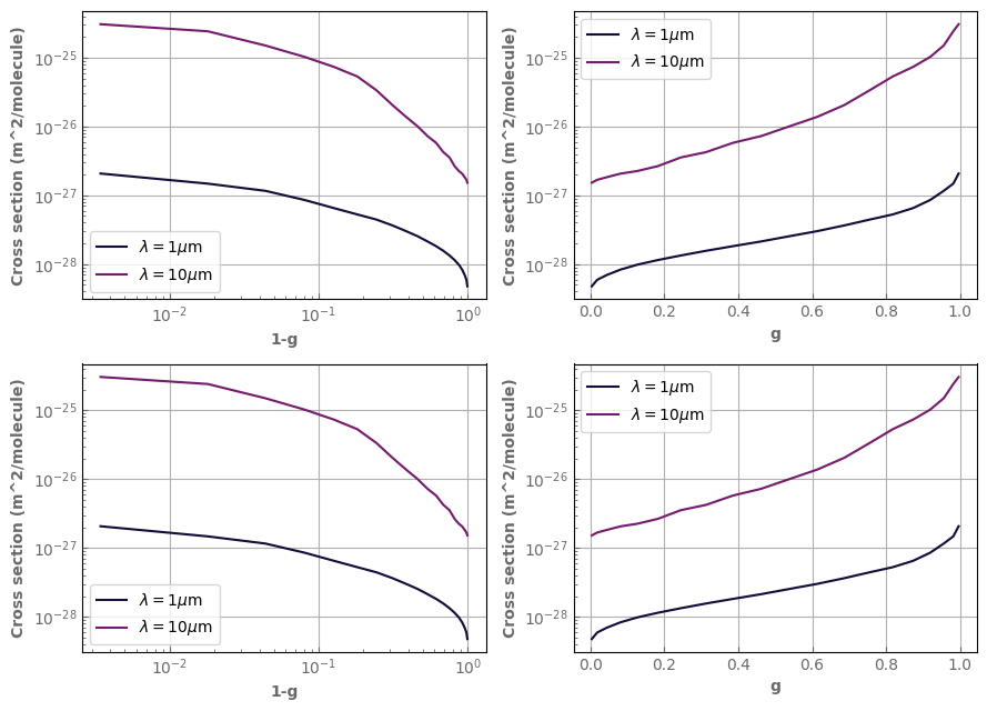
The g distribution is shown with plot_distrib. Notice that when you ask for a log scale in g, we switch to 1-g as it is the most relevant quantity to look at in log.
[22]:
p_plot=1.e5
t_plot=1000.
fig,axs=plt.subplots(2,2,sharex=False,sharey=False,figsize=(9,6.5))
h2o_ktab_SI.plot_distrib(axs[0,0],p=p_plot,t=t_plot,wl=1.0,yscale='log',xscale='log',label=r'$\lambda=1\mu$m')
h2o_ktab_SI.plot_distrib(axs[0,0],p=p_plot,t=t_plot,wl=10.,yscale='log',xscale='log',label=r'$\lambda=10\mu$m')
h2o_ktab_SI.plot_distrib(axs[1,0],p=p_plot,t=t_plot,wl=1.0,xscale='log',label=r'$\lambda=1\mu$m')
h2o_ktab_SI.plot_distrib(axs[1,0],p=p_plot,t=t_plot,wl=10.,xscale='log',label=r'$\lambda=10\mu$m')
h2o_ktab_SI.plot_distrib(axs[0,1],p=p_plot,t=t_plot,wl=1.0,yscale='log',label=r'$\lambda=1\mu$m')
h2o_ktab_SI.plot_distrib(axs[0,1],p=p_plot,t=t_plot,wl=10.,yscale='log',label=r'$\lambda=10\mu$m')
h2o_ktab_SI.plot_distrib(axs[1,1],p=p_plot,t=t_plot,wl=1.0,label=r'$\lambda=1\mu$m')
h2o_ktab_SI.plot_distrib(axs[1,1],p=p_plot,t=t_plot,wl=10.,label=r'$\lambda=10\mu$m')
for axs in axs:
    for ax in axs:
        ax.legend()
#ax.set_ylim(bottom=1.e-37)
fig.tight_layout()

Interpolating and remapping tables
Basic interpolation
To get the value of the cross section of the molecule or mix described by our Ktable() object, we can use:
self.interpolate_kdata(logp_array=None,t_array=None,log_interp=None,wngrid_limit=None)
This returns the cross section of the molecule along a LogP-T profile specified by logp_array and t_array. This returns an array of shape (logp_array.size, self.Nw, self.Ng), i.e (number of PT points, number of wavenumber points, number of g-points). logp_arrayand t_arraymust have the same size.
It also works if logp_array and/or t_array are floats
Important
Notice that the input is always in Log10(Pressure) because this is the quantity used for the interpolation
See also
exo_k.data_table.Data_table.interpolate_kdata() for details on arguments and options.
[23]:
logp=3.
Temp=1000.
tmp_opa=h2o_ktab_SI.interpolate_kdata(logp,Temp)
print(tmp_opa.shape)
print(tmp_opa)
(1, 1538, 20)
[[[1.57577243e-26 1.70593813e-26 1.71642784e-26 ... 4.95008363e-22
   8.13668554e-22 9.35286142e-22]
  [2.90167053e-26 4.18911348e-26 4.71088691e-26 ... 8.99173698e-23
   4.25319413e-22 6.23065168e-22]
  [5.81193968e-27 5.82883586e-27 5.92632233e-27 ... 1.21096603e-25
   3.52299381e-25 4.86654868e-25]
  ...
  [2.43561538e-34 3.12899011e-34 3.55619421e-34 ... 2.18003828e-33
   2.92876500e-33 3.94600721e-33]
  [2.71942214e-34 3.29638704e-34 3.74713705e-34 ... 2.21029744e-33
   3.13286094e-33 5.08112258e-33]
  [2.86054904e-34 3.25393178e-34 3.70676091e-34 ... 2.45139953e-33
   3.46404319e-33 7.47015700e-33]]]
[24]:
logp_array=np.linspace(1.,6.,6)
t_array=[1000. for logp in logp_array]
tmp_opa=h2o_ktab_SI.interpolate_kdata(logp_array,t_array)
print(tmp_opa.shape)
(6, 1538, 20)
Interpolation options
The default interpolation scheme interpolates log(kdata). This can be changed directly using the log_interp=False keyword. But the default behavior can also be changed using Settings().set_log_interp. The keyword always supercedes the default behavior.
[25]:
logp=3.
Temp=1000.
tmp_opa_lin1=h2o_ktab_SI.interpolate_kdata(logp,Temp,log_interp=False)
[26]:
xk.Settings().set_log_interp(False)
logp=3.
Temp=1000.
tmp_opa_lin2=h2o_ktab_SI.interpolate_kdata(logp,Temp)
np.sum(tmp_opa_lin2-tmp_opa_lin1)
xk.Settings().set_log_interp(True) ## let's go back to default behavior
Linear interpolation is of course faster, but is believed to be less accurate.
[27]:
logp=3.
Temp=1000.
%timeit -n 100 -r 2 h2o_ktab_SI.interpolate_kdata(logp,Temp,log_interp=True)
%timeit -n 100 -r 2 h2o_ktab_SI.interpolate_kdata(logp,Temp,log_interp=False)
465 µs ± 21.8 µs per loop (mean ± std. dev. of 2 runs, 100 loops each)
174 µs ± 450 ns per loop (mean ± std. dev. of 2 runs, 100 loops each)
[28]:
logp=3.
Temp=1000.
wn_range=[6000.,5000.] # does not need to be sorted
%timeit -n 100 -r 2 h2o_ktab_SI.interpolate_kdata(logp,Temp,wngrid_limit=wn_range,log_interp=True)
%timeit -n 100 -r 2 h2o_ktab_SI.interpolate_kdata(logp,Temp,wngrid_limit=wn_range,log_interp=False)
tmp_opa=h2o_ktab_SI.interpolate_kdata(logp,Temp,wngrid_limit=wn_range)
print(tmp_opa.shape)
print(tmp_opa)
164 µs ± 29.6 µs per loop (mean ± std. dev. of 2 runs, 100 loops each)
95.3 µs ± 5.63 µs per loop (mean ± std. dev. of 2 runs, 100 loops each)
(1, 54, 20)
[[[4.07753036e-29 6.85197398e-29 1.02732246e-28 ... 2.41869028e-25
   4.85016488e-25 1.14633633e-24]
  [5.57875921e-29 7.97288442e-29 1.21104087e-28 ... 3.42969506e-25
   1.22902497e-24 2.53733317e-24]
  [6.17042832e-29 9.10883868e-29 1.31081205e-28 ... 3.53333315e-25
   8.73232110e-25 3.80127738e-24]
  ...
  [2.02444510e-30 3.93145431e-30 5.47901786e-30 ... 2.32477558e-27
   7.86972907e-27 3.78365657e-26]
  [2.33493343e-30 3.54354098e-30 4.84518937e-30 ... 2.32501304e-27
   6.12582068e-27 2.35847913e-26]
  [2.50675050e-30 3.68390571e-30 4.92245284e-30 ... 2.94029197e-27
   1.10535798e-26 4.63705729e-26]]]
(Log P, T) grid Remapping
If for computational efficiency reason we just want to use a subset of the (Log P, T) grid, we can remap the table. This will modify the Table in place. So we might want to make a copy before.
[29]:
Small_Grid_h2o_ktab=h2o_ktab_SI.copy()
logp_array=np.arange(6.)
t_array=np.linspace(200.,1000.,9)

Small_Grid_h2o_ktab.remap_logPT(logp_array=logp_array,t_array=t_array)
Small_Grid_h2o_ktab
[29]:
        file         : /builds/jleconte/exo_k-public/data/corrk/H2O_R300_0.3-50mu.ktable.SI.h5
        molecule     : H2O
        p grid       : [1.e+00 1.e+01 1.e+02 1.e+03 1.e+04 1.e+05]
        p unit       : Pa
        t grid   (K) : [ 200.  300.  400.  500.  600.  700.  800.  900. 1000.]
        wn grid      : [  199.90345491   200.56979976   201.23836576 ... 33057.12210094
 33167.31250795 33277.87021631]
        wn unit      : cm^-1
        kdata unit   : m^2/molecule
        weights      : [0.008807   0.02030071 0.03133602 0.04163837 0.05096506 0.05909727
 0.06584432 0.07104805 0.07458649 0.07637669 0.07637669 0.07458649
 0.07104805 0.06584432 0.05909727 0.05096506 0.04163837 0.03133602
 0.02030071 0.008807  ]
        data oredered following p, t, wn, g
        shape        : [   6    9 1538   20]
Remapping in g-space
Sometimes, we also want to reduce the number of g-points, or combine two tables with different g-quadratures. For this we can use the following:
[30]:
# simple function to compute a set of gauss legendre points and weights
from exo_k.util.interp import gauss_legendre
weights, ggrid, gedges=gauss_legendre(8)
ggrid
[30]:
array([0.01985507, 0.10166676, 0.2372338 , 0.40828268, 0.59171732,
       0.7627662 , 0.89833324, 0.98014493])
[31]:
h2o_ktab_8g=h2o_ktab_SI.copy()
h2o_ktab_8g.remap_g(ggrid=ggrid, weights=weights)
h2o_ktab_8g
[31]:
        file         : /builds/jleconte/exo_k-public/data/corrk/H2O_R300_0.3-50mu.ktable.SI.h5
        molecule     : H2O
        p grid       : [1.00000000e+00 2.15443469e+00 4.64158883e+00 1.00000000e+01
 2.15443469e+01 4.64158883e+01 1.00000000e+02 2.15443469e+02
 4.64158883e+02 1.00000000e+03 2.15443469e+03 4.64158883e+03
 1.00000000e+04 2.15443469e+04 4.64158883e+04 1.00000000e+05
 2.15443469e+05 4.64158883e+05 1.00000000e+06 2.15443469e+06
 4.64158883e+06 1.00000000e+07]
        p unit       : Pa
        t grid   (K) : [ 100.  200.  300.  400.  500.  600.  700.  800.  900. 1000. 1100. 1200.
 1300. 1400. 1500. 1600. 1700. 1800. 1900. 2000. 2200. 2400. 2600. 2800.
 3000. 3200. 3400.]
        wn grid      : [  199.90345491   200.56979976   201.23836576 ... 33057.12210094
 33167.31250795 33277.87021631]
        wn unit      : cm^-1
        kdata unit   : m^2/molecule
        weights      : [0.05061427 0.11119052 0.15685332 0.18134189 0.18134189 0.15685332
 0.11119052 0.05061427]
        data oredered following p, t, wn, g
        shape        : [  22   27 1538    8]
The table now has only 8 g points. You can of course specify custom g-points and weights if you want.
Extending the spectral range
As we will see afterwards, we need tables to have the same spectral grid to be able to combine them. If they cover the same spectral range, but with different resolution, the solution is to bin them down as explained a few sections down. If, however, we want to combine molecules that are absorbing in rather different part of the spectrum, we may often encounter tables that cover only the spectral region where each molecule has a significant absorption.
To circumvent this issue, exo_k allows you to extend the spectral range of your table adding a null opacity (or a very small one if one wants to use log interpolation afterwards) in the new spectral bins. This can be done as follows. It changes the table in place.
There are 3 options to specify the left and/or right extension of the spectral grid:
The
wngrid_left/rightkeyword allows you to specify the center of the new bins. The edges are computed automatically. This option is most useful withXtablesfor which you most want to control the center of the bins.The
wnedges_left/rightkeyword allows you to specify the the edges of the new spectral bin. Bin centers are computed automatically. This option is most useful withKtablesfor which you most want to control the edges of the bins. Since we are re-using the last wnedges on the left and right of the current grid, the user only needs to specifyNnew values to createNnew bins.You can specify both at the same time.
Warning
The user must make sure that the new left and right wavenumber grids do not overlap with the current one. If both wnedges and wngrids are specified, the user should also make sure that there is one (and only one) wavenumber point between each pair of wnegdes points.
[32]:
large_spectral_range_h2o=h2o_ktab_SI.copy()
new_wn_points_left=np.linspace(10,190,20)
new_wn_edges_left=np.linspace(5,185,20)
new_wn_points_right=np.linspace(33400,50000,20)
new_wn_edges_right=np.linspace(33450,50050,20)

# specifying only wngrid
#large_spectral_range_h2o.extend_spectral_range(wngrid_left=new_wn_points_left, wngrid_right=new_wn_points_right, remove_zeros=True)
large_spectral_range_h2o.extend_spectral_range(wngrid_left=new_wn_points_left, wnedges_left=new_wn_edges_left,
                                               wngrid_right=new_wn_points_right, wnedges_right=new_wn_edges_right, remove_zeros=True)
#large_spectral_range_h2o.extend_spectral_range( wnedges_left=new_wn_edges_left,wnedges_right=new_wn_edges_right, remove_zeros=True)
print('Old wn grid: ',h2o_ktab_SI.wns)
print('New wn grid: ',large_spectral_range_h2o.wns)
print('Old wn edges: ',h2o_ktab_SI.wnedges)
print('New wn edges: ',large_spectral_range_h2o.wnedges)

p_plot=1.e5
t_plot=1000.
fig,ax=plt.subplots(1,1,sharex=False,sharey=False,figsize=(6,4.5))
large_spectral_range_h2o.plot_spectrum(ax,p=p_plot,t=t_plot,g=1.,yscale='log',xscale='log',color='black',linestyle='dashed',label='after extension')
h2o_ktab_SI.plot_spectrum(ax,p=p_plot,t=t_plot,g=1.,label='before extension')
ax.legend()
fig.tight_layout()
Old wn grid:  [  199.90345491   200.56979976   201.23836576 ... 33057.12210094
 33167.31250795 33277.87021631]
New wn grid:  [1.00000000e+01 1.94736842e+01 2.89473684e+01 ... 4.82526316e+04
 4.91263158e+04 5.00000000e+04]
Old wn edges:  [  199.57138937   200.23662733   200.90408276 ... 33112.21730444
 33222.59136213 33333.33333333]
New wn edges:  [5.00000000e+00 1.44736842e+01 2.39473684e+01 ... 4.83026316e+04
 4.91763158e+04 5.00500000e+04]

Clipping data to a given spectral range
If for effciency reasons you want to only deal with a small part of the spectral domain, you can use the Ktable.clip_spectral_range(wl_range= , wn_range= ) method with either a wavelength range (wl_rangein microns) or a wavenumber range (wn_range in cm^-1). Data outside this range will be removed from the table.
Binning down a Ktable
We now get to one of the core features of exo_k: we want to create a new Ktable() object with just the spectral resolution we need in the model we want to run (whether it is a Global Climate Model, a 1D climate model, or a simple forward model for a retrieval).
You first need to provide a grid, wnedges, containing the edges of the new wavenumber bins. So the final Ktable will have a spectral dimension with size wnedges.size-1.
You can of course provide any custom grid you want. But if you want a grid at fixed resolution you can use the following
xk.wavenumber_grid_R(min_wavenumber, max_wavenumber, R)
where \(R=\frac{\nu}{\delta \nu}\).
[33]:
R=10
wavenumber_grid=xk.wavenumber_grid_R(200.,10000.,R)
wavenumber_grid
[33]:
array([  200.        ,   221.03418362,   244.28055163,   269.97176152,
         298.36493953,   329.74425414,   364.42376008,   402.75054149,
         445.1081857 ,   491.92062223,   543.65636569,   600.83320479,
         664.02338455,   733.85933352,   811.03999337,   896.33781407,
         990.60648488,  1094.78947835,  1209.92949288,  1337.17888846,
        1477.81121979,  1633.23398251,  1805.00269989,  1994.83649096,
        2204.63527613,  2436.49879214,  2692.747607  ,  2975.94634497,
        3288.92935422,  3634.82907389,  4017.10738464,  4439.59025629,
        4906.50603942,  5422.52778413,  5992.82000948,  6623.09039174,
        7319.64688874,  8089.46087201,  8940.23689866,  9880.48982111,
       10000.        ])
Then we just need to use the bin_down(wnedges) method. However, bin_down modifies the Ktable() in place. So again, if we want to keep the original one in memory, we just copy it or use bin_down_cp.
Optional keywords can be weights= and ggrid= where you can provide the weights you want (and the corresponding g points). In general, for an LMDZ user, just input the values inside g.dat (except for the final zero) in a w_array, and use weights=w_array. If you want gauss legendre weights, you can have a look at exo_k.gauss_legendre in the index.
See also
exo_k.ktable.Ktable.bin_down() bin_down_cp()
for details on arguments and options.
It should only take a few seconds. (However, the bigger the final resolution wanted, the longer it takes).
[34]:
start=time.time()
LowRes_h2o_ktab=h2o_ktab_SI.bin_down_cp(wavenumber_grid)
end=time.time()
print('computation time=',end-start,'s')
LowRes_h2o_ktab
computation time= 14.740747690200806 s
[34]:
        file         : /builds/jleconte/exo_k-public/data/corrk/H2O_R300_0.3-50mu.ktable.SI.h5
        molecule     : H2O
        p grid       : [1.00000000e+00 2.15443469e+00 4.64158883e+00 1.00000000e+01
 2.15443469e+01 4.64158883e+01 1.00000000e+02 2.15443469e+02
 4.64158883e+02 1.00000000e+03 2.15443469e+03 4.64158883e+03
 1.00000000e+04 2.15443469e+04 4.64158883e+04 1.00000000e+05
 2.15443469e+05 4.64158883e+05 1.00000000e+06 2.15443469e+06
 4.64158883e+06 1.00000000e+07]
        p unit       : Pa
        t grid   (K) : [ 100.  200.  300.  400.  500.  600.  700.  800.  900. 1000. 1100. 1200.
 1300. 1400. 1500. 1600. 1700. 1800. 1900. 2000. 2200. 2400. 2600. 2800.
 3000. 3200. 3400.]
        wn grid      : [ 210.51709181  232.65736762  257.12615657  284.16835052  314.05459683
  347.08400711  383.58715079  423.9293636   468.51440396  517.78849396
  572.24478524  632.42829467  698.94135904  772.44966345  853.68890372
  943.47214947 1042.69798161 1152.35948561 1273.55419067 1407.49505412
 1555.52260115 1719.1183412  1899.91959542 2099.73588355 2320.56703413
 2564.62319957 2834.34697599 3132.4378496  3461.87921405 3825.96822926
 4228.34882046 4673.04814786 5164.51691178 5707.67389681 6307.95520061
 6971.36864024 7704.55388037 8514.84888534 9410.36335988 9940.24491055]
        wn unit      : cm^-1
        kdata unit   : m^2/molecule
        weights      : [0.008807   0.02030071 0.03133602 0.04163837 0.05096506 0.05909727
 0.06584432 0.07104805 0.07458649 0.07637669 0.07637669 0.07458649
 0.07104805 0.06584432 0.05909727 0.05096506 0.04163837 0.03133602
 0.02030071 0.008807  ]
        data oredered following p, t, wn, g
        shape        : [22 27 40 20]
[35]:
p_plot=1.e0
t_plot=300.
fig,axs=plt.subplots(1,2,sharex=False,sharey=False)
h2o_ktab_SI.plot_spectrum(axs[0],p=p_plot,t=t_plot,g=1.,yscale='log',xscale='log',label='Original data')
LowRes_h2o_ktab.plot_spectrum(axs[0],p=p_plot,t=t_plot,g=1.,label='Binned data')
h2o_ktab_SI.plot_spectrum(axs[1],p=p_plot,t=t_plot,g=1.,yscale='log',xscale='log',label='Original data')
LowRes_h2o_ktab.plot_spectrum(axs[1],p=p_plot,t=t_plot,g=1.,label='Binned data')
axs[1].set_xlim(left=1.,right=6.)
axs[1].set_xscale('linear')
for ax in axs:
    ax.legend()
fig.tight_layout()

Rescaling and mixing Ktables
The Ktable we have seen up to now contain opacity data (in terms of cross section in surface per molecule) for pure species. To create a mix, you can dilute your tables with (multiply by) the Volume mixing ratio of the relevant species and add them.
Important
Although we are using the ‘+’ sign, the tables are actually combined using the Random overlap method.
Warning
Ktable`s should have the same dimensions and grids to be combined. For efficiency, the code only checks whether the dimensions are the same (and raises a `TypeError if they are not). The user should make sure the grids are the same as well.
[36]:
h2o=xk.Ktable('H2O_R300_0.3-50mu.ktable.SI', remove_zeros=True)
co2=xk.Ktable('CO2_R300_0.3-50mu.ktable.SI', remove_zeros=True)
for ktab in [co2,h2o]:
    ktab.remap_logPT(logp_array=np.arange(0,5),t_array=np.arange(200.,500.,50.))
start=time.time()
mix=0.01*h2o+co2*0.02
print('Mixing time=',time.time()-start,'s')
Mixing time= 2.094414472579956 s
[37]:
p_plot=1.e0
t_plot=300.
fig,ax=plt.subplots(1,1,sharex=False,sharey=False)
h2o.plot_spectrum(ax,p=p_plot,t=t_plot,g=1.,x=0.01,yscale='log',xscale='log',label='H2O')
co2.plot_spectrum(ax,p=p_plot,t=t_plot,g=1.,x=0.01,label='CO2')
mix.plot_spectrum(ax,p=p_plot,t=t_plot,g=1.,yscale='log',xscale='log',label='mix')
ax.set_ylim(bottom=1.e-36)
ax.legend()
fig.tight_layout()

Important
For the moment, the Ktable for the mix inherits attributes (such as the name of the molecule) from the most leftward Ktable in the operation.
The renormalization operation also accepts an array of volume mixing ratio, but only if it has the dimensions (Number of P points, number of T points).
[38]:
x_h2o=np.array([0.01+0.02*logP+0.00001*T for logP in h2o.logpgrid for T in h2o.tgrid]).reshape((h2o.Np,h2o.Nt))
mix=x_h2o*h2o+co2*0.02
Dealing with mixes: The Kdatabase() object
Loading a Kdatabase() object
Global loading from files
A Kdatabase() object mainly contains a dictionary of Ktable() objects identified by the name of their molecule (in the attribute self.ktables, but they can be accessed with self['mol_name']). In addition, most of the attributes of the Ktable() are reloaded as attributes of Kdatabase().
To load a database, just specify a list of molecules and a string filter that is common to all your filenames.
For details on the available arguments and options, check-out :func:exo_k.kdatabase.Kdatabase.
[39]:
molecs=['H2O','CO2']
filt='R300_0.3-50mu.ktable.SI'
database=xk.Kdatabase(molecs, filt)
database
[39]:
The available molecules are:
H2O->/builds/jleconte/exo_k-public/data/corrk/H2O_R300_0.3-50mu.ktable.SI.h5
CO2->/builds/jleconte/exo_k-public/data/corrk/CO2_R300_0.3-50mu.ktable.SI.h5
All tables share a common spectral grid
All tables share a common logP-T grid
All tables share a common p unit
All tables share a common kdata unit
It will look for files starting with the molecule names, followed by _, ., or -, and containing the filters.
If you want the moleculer name to be followed by something else than these characters, then just change the setting by using the xk.Settings().set_delimiters method.
Of course, this is unpractical when you do not have a homogeneous set of Ktables to start with. Then you can just feed a dictionary of molecules with the associated files path.
[40]:
database=xk.Kdatabase({'H2O':datapath + 'corrk/H2O_R300_0.3-50mu.ktable.TauREx.h5',
                       'CO2':datapath + 'corrk/CO2_R300_0.3-50mu.ktable.SI.h5'},
                       p_unit='Pa', kdata_unit='m^2/molecule')
database
[40]:
The available molecules are:
H2O->../data/corrk/H2O_R300_0.3-50mu.ktable.TauREx.h5
CO2->../data/corrk/CO2_R300_0.3-50mu.ktable.SI.h5
All tables share a common spectral grid
All tables share a common logP-T grid
All tables share a common p unit
All tables share a common kdata unit
Warning
The latest release of Exomol data is using a new convention to write molecule names in filenames to include isotopologues. For example, the name of a file describing the water molecule now starts with ‘1H2-16O’ instead of ‘H2O’. To use these, use the new name in the method call (database=xk.Kdatabase([‘1H2-16O’,’12C-16O2’], filt)). However, be aware that inside the database object, individual `Ktable`s are recognized and called by the name of the molecule that is stored inside the file (‘H2O’ and ‘CO2’ in our case; see the accessing individual `Ktable`s section below).
For FITS and Nemesis formats that do not yet include the molecule name inside the file, we recommend that you use the second loading method: database=xk.Kdatabase({‘H2O’: datapath + ‘corrk/1H2-16O__POKAZATEL__R1000_0.3-50mu.ktable.ARCiS.fits’, etc.}).
Adding individual, already-loaded Ktables
Sometimes, you want to modify/remap/bin_down your Ktables before loading it into a Kdatabase. However, you do not necessarily want to have to store these intermediate steps into a file to read it into a database as described above.
To do this, you can add one or several Ktable using the add_ktables(*ktables) method. If you want to start from scratch, you’ll need to create an empty Kdatabase as follows.
[41]:
database=xk.Kdatabase(None) # create empty database
print(database)

h2o=xk.Ktable('H2O_R300_0.3-50mu.ktable.SI', remove_zeros=True)
co2=xk.Ktable('CO2_R300_0.3-50mu.ktable.SI', remove_zeros=True)
co2.remap_logPT(logp_array=np.arange(0,5),t_array=np.arange(200.,500.,50.))

database.add_ktables(h2o, co2)
print(database)
The available molecules are:
All tables share a common spectral grid
All tables share a common logP-T grid
All tables share a common p unit
All tables share a common kdata unit

Careful, not all tables have the same logPT grid.
                        You'll need to use remap_logPT
The available molecules are:
H2O->/builds/jleconte/exo_k-public/data/corrk/H2O_R300_0.3-50mu.ktable.SI.h5
CO2->/builds/jleconte/exo_k-public/data/corrk/CO2_R300_0.3-50mu.ktable.SI.h5
All tables share a common spectral grid
All tables do NOT have common logP-T grid
You will need to run remap_logPT to perform some operations
All tables share a common p unit
All tables share a common kdata unit
Dealing with inhomogeneous databases
As we are loading Ktables from various possible sources, that we may have modified however we like, we are bound to end up with a inhomogeneous database because all the Ktable:
do not have the same datatype.
do not have the same weights and g grid,
do not have the same logP-T grid,
do not have the same spectral grid,
do not have the same units
For the moment, a Kdatabase needs to be homogeneous to be used to create mixes or compute forward models (see below).
The 1st issue is due to the fact that exo_k can handle other types of data (e.g. Xtable that are regular cross section tables; see dedicated section below). Although these data types can be handled in a database, a Kdatabase can only deal with a single type at a time. Loading different types will result in an error.
The 2nd issue is delicate because there are no easy way to accurately re-interpolate a Ktable on a different g grid. So for the moment, there is no way to remedy this. The user needs to provide Ktable with the same g grid and weights. Loading tables with different g grids will result in an error.
The remaining issues are easily handled by following the suggestion in the warning message (see above):
Using
Kdatabase.remap_logPT(logp_array= , t_array= )will homogenize the log P-T grid by interpolating (in place) all theKtablesto a common grid.Using
Kdatabase.bin_down(wnedges= , **kwargs)will homogenize the spectral grid by binning down (in place) all theKtablesto a common grid.If you are using cross sections, the spectral grid can be homogenized using
Kdatabase.sample(wngrid= )instead of bin_down (see below).All the
Ktables can be converted to the same units usingKdatabase.convert_p_unit()andKdatabase.convert_kdata_unit(), or directlyKdatabase.convert_to_mks()
[42]:
print(database)
print('remapping...')
database.remap_logPT(logp_array=np.arange(0,5),t_array=np.arange(200.,500.,50.))
print(database)
The available molecules are:
H2O->/builds/jleconte/exo_k-public/data/corrk/H2O_R300_0.3-50mu.ktable.SI.h5
CO2->/builds/jleconte/exo_k-public/data/corrk/CO2_R300_0.3-50mu.ktable.SI.h5
All tables share a common spectral grid
All tables do NOT have common logP-T grid
You will need to run remap_logPT to perform some operations
All tables share a common p unit
All tables share a common kdata unit

remapping...
The available molecules are:
H2O->/builds/jleconte/exo_k-public/data/corrk/H2O_R300_0.3-50mu.ktable.SI.h5
CO2->/builds/jleconte/exo_k-public/data/corrk/CO2_R300_0.3-50mu.ktable.SI.h5
All tables share a common spectral grid
All tables share a common logP-T grid
All tables share a common p unit
All tables share a common kdata unit
Warning
A Ktable is not deep copied when loaded into a database! Modifying the database inplace thus modifies the original table as well.
[43]:
# See how the values in the P and T grids have changed
# compared to their values in the previous section.
h2o
[43]:
        file         : /builds/jleconte/exo_k-public/data/corrk/H2O_R300_0.3-50mu.ktable.SI.h5
        molecule     : H2O
        p grid       : [1.e+00 1.e+01 1.e+02 1.e+03 1.e+04]
        p unit       : Pa
        t grid   (K) : [200. 250. 300. 350. 400. 450.]
        wn grid      : [  199.90345491   200.56979976   201.23836576 ... 33057.12210094
 33167.31250795 33277.87021631]
        wn unit      : cm^-1
        kdata unit   : m^2/molecule
        weights      : [0.008807   0.02030071 0.03133602 0.04163837 0.05096506 0.05909727
 0.06584432 0.07104805 0.07458649 0.07637669 0.07637669 0.07458649
 0.07104805 0.06584432 0.05909727 0.05096506 0.04163837 0.03133602
 0.02030071 0.008807  ]
        data oredered following p, t, wn, g
        shape        : [   5    6 1538   20]
Accessing individual Ktables
A Kdatabase is essentially a dictionary and individual Ktable objects can be accessed using the molecule name as a key. When adding Ktables one by one, the molecule name used as a key is inherited from the Ktable.mol attribute. If you are loading a new Ktable with a molecule name that is already in the database, the latter will be replaced.
[44]:
database['H2O'].filename
[44]:
'/builds/jleconte/exo_k-public/data/corrk/H2O_R300_0.3-50mu.ktable.SI.h5'
Warning
You cannot load a new table this way!
`python
database['SiO']=SiO_ktable
TypeError: 'Kdatabase' object does not support item assignment
`
Create a Ktable() for a mix of gases
One of the main interests of databases is to actually be able to create new correlated-k tables for mixtures of gases (the other being running a full atmospheric model as we will see at the end).
Just create a dictionary with the names of the molecules and the corresponding volume mixing ratios. Notice that the sum of the mixing ratios does not need to be equal to one. In that case, it is assumed that the rest of the gas is composed of radiatively inactive species. Then, the opacity given is in m^2 per total number of molecules (couting the inactive ones).
If a molecule is not in the database, it will just be considered radiatively inactive.
[45]:
molecs=['H2O','CO2']
suffix='R300_0.3-50mu.ktable.SI'
database=xk.Kdatabase(molecs,suffix)

composition={'H2O':0.001,'CO2':400.e-6,'N2':'background'}

start=time.time()
mixH2O_CO2=database.create_mix_ktable(composition)

mixH2O_CO2.write_hdf5(datapath + 'corrk/mix_H2O_CO2')

end=time.time()
print("computation time ",end - start,'s')
computation time 29.7729012966156 s
Here, the 'N2':'background'in the composition dictionary tells the code that N2 is the background ‘filler’ gas. So whatever the vmr given before, N2 will be adjusted to get a total vmr of 1. Because N2 is not in the database (because it does not have any strong lines), its opacity will however not be considered.
(Why doing this you might ask? Well, here including N2 does not change anything as it is considered transparent anyway. This will become important however when we will deal with atmospheric models where including N2 will allow us to have the right mean molecular weight for the atmosphere).
[46]:
ptest=1.e4
ttest=300.
fig,axs=plt.subplots(1,2,sharex=True,sharey=True)
for species,x in composition.items():
  if x != 'background':
    database[species].plot_spectrum(axs[0],p=ptest,t=ttest,g=1.,x=x,linestyle='dashed',yscale='log')
    database[species].plot_spectrum(axs[1],p=ptest,t=ttest,g=0.,x=x,linestyle='dashed',yscale='log')
mixH2O_CO2.plot_spectrum(axs[0],p=ptest,t=ttest,g=1.)
mixH2O_CO2.plot_spectrum(axs[1],p=ptest,t=ttest,g=0.)
axs[0].set_title('g=1')
axs[1].set_title('g=0')
for ax in axs :
    ax.set_xscale('log')
    ax.label_outer()
    ax.set_ylim(bottom=1.e-40)
fig.tight_layout()

Binning down a Kdatabase()
Just like Ktable() objects, you can change the spectral resolution of an entire database with the same bin_down(wnedges) method. It will be applied to all ktables in place (weights keyword available as well).
[47]:
R=10
wavenumber_grid=xk.wavenumber_grid_R(200.,10000.,R)
database.bin_down(wavenumber_grid)
Notice how the resolution has changed below when we run the exact same code.
[48]:
ptest=1.e4
ttest=300.

fig,axs=plt.subplots(1,2,sharex=True,sharey=True)
for species,x in composition.items():
  if x != 'background':
    database[species].plot_spectrum(axs[0],p=ptest,t=ttest,g=1.,x=x,linestyle='dashed',label=species)
    database[species].plot_spectrum(axs[1],p=ptest,t=ttest,g=0.,x=x,linestyle='dashed',label=species)
mixH2O_CO2.plot_spectrum(axs[0],p=ptest,t=ttest,g=1.,label='mix')
mixH2O_CO2.plot_spectrum(axs[1],p=ptest,t=ttest,g=0.,label='mix')
axs[0].set_title('g=1')
axs[1].set_title('g=0')
for ax in axs :
    ax.set_xscale('log')
    ax.set_yscale('log')
    ax.label_outer()
    ax.set_ylim(bottom=1.e-40)
    ax.legend()
fig.tight_layout()

Loading and creating correlated-k tables to use with LMDZ GCM
Creating new corr-k for LMDZ-GCM
exo_k has also been designed to create corr-k tables to be used with the LMDZ gcm.
To produce a LMDZ usable directory with the corr-k and all the supporting files, nothing is simpler.
Important
This section only deals with corr-k tables without variable gases. For these, we need to deal with gas mixes and Ktable5D that are discussed a little further down.
First, let’s create a grid for our IR and VI channels and create our two ktables.
[49]:
R=10
IR_grid=xk.wavenumber_grid_R(220.,10000.,R)
VI_grid=xk.wavenumber_grid_R(5200.,33000.,R)

IR_h2o_ktab=h2o_ktab_SI.bin_down_cp(IR_grid)

VI_h2o_ktab=h2o_ktab_SI.bin_down_cp(VI_grid)
Once your low resolution corrk table has been produced, just run
[50]:
IR_h2o_ktab.write_LMDZ(datapath + 'corrk/lmdz/new_h2o_corrk',band='IR')
VI_h2o_ktab.write_LMDZ(datapath + 'corrk/lmdz/new_h2o_corrk',band='VI')
Should you care about units?
Actually… no! Because we have tracked units from the beginning, and we know LMDZ likes ktables in cm^2/molec and pressures in log mBar, the conversion has been done automatically for you.
The LMDZ aficionados may have noticed that in the corrk/new_h2o_corrk directory, two subdirectories have been created with the names IR self.Nw and VI self.Nw that contain the corr-k tables whereas we would like a single directory called Number_of_IR_bins x Number_of_VI_bins. Then just run:
[51]:
xk.finalize_LMDZ_dir(datapath + 'corrk/lmdz/new_h2o_corrk',IR_h2o_ktab.Nw,VI_h2o_ktab.Nw)
Everything went ok. Your ktable is in: ../data/corrk/lmdz/new_h2o_corrk/39x19
You'll probably need to add Q.dat before using it though!
You just have to create a Q.dat file in the directory and you are good to run LMDZ with new corrk. If you do not know what I am talking about, you have not been using the LMDZ GCM long enough!
Loading existing LMDZ corr-k tables
To load a LMDZ corr-k table, the initialization method needs some more information:
The directory to use (
path=)The resolution (
res=)Whether you want to load the ‘IR’ or ‘VI’ band (
band=)
The mol keyword can be given to specify which species is described. This will be useful for mixes.
Here, if you do not specify units, you will keep the LMDZ ones (cm^2 and mBar). But we advise to use the SI units. In particular because our radiative transfer method use SI units.
[52]:
IR_h2o_ktab=xk.Ktable(path=datapath + 'corrk/lmdz/new_h2o_corrk',res='39x19',band='IR',mol='H2O',
                kdata_unit='m^2',p_unit='Pa')
print(IR_h2o_ktab)
        file         : ../data/corrk/lmdz/new_h2o_corrk
        molecule     : H2O
        p grid       : [1.00000000e+00 2.15443469e+00 4.64158883e+00 1.00000000e+01
 2.15443469e+01 4.64158883e+01 1.00000000e+02 2.15443469e+02
 4.64158883e+02 1.00000000e+03 2.15443469e+03 4.64158883e+03
 1.00000000e+04 2.15443469e+04 4.64158883e+04 1.00000000e+05
 2.15443469e+05 4.64158883e+05 1.00000000e+06 2.15443469e+06
 4.64158883e+06 1.00000000e+07]
        p unit       : Pa
        t grid   (K) : [ 100.  200.  300.  400.  500.  600.  700.  800.  900. 1000. 1100. 1200.
 1300. 1400. 1500. 1600. 1700. 1800. 1900. 2000. 2200. 2400. 2600. 2800.
 3000. 3200. 3400.]
        wn grid      : [ 231.56880099  255.92310439  282.83877223  312.58518557  345.46005652
  381.79240782  421.94586586  466.32229996  515.36584436  569.56734336
  629.46926376  695.67112414  768.83549494  849.69462979  939.05779409
 1037.81936442 1146.96777977 1267.59543418 1400.90960974 1548.24455953
 1711.07486126 1891.03017532 2089.91155497 2309.7094719  2552.62373755
 2821.08551953 3117.78167359 3445.68163456 3808.06713546 4208.56505219
 4651.18370251 5140.35296264 5680.96860295 6278.44128649 6938.75072067
 7668.50550426 8475.00926841 9366.33377387 9917.13029426]
        wn unit      : cm^-1
        kdata unit   : m^2/molecule
        weights      : [0.008807   0.02030071 0.03133602 0.04163837 0.05096506 0.05909727
 0.06584432 0.07104805 0.07458649 0.07637669 0.07637669 0.07458649
 0.07104805 0.06584432 0.05909727 0.05096506 0.04163837 0.03133602
 0.02030071 0.008807  ]
        data oredered following p, t, wn, g
        shape        : [22 27 39 20]
Creating a LMDZ corr-k with a variable gas from a Kdatabase: the Ktable5d
Here, we will finally see one of the strengths of Kdatabase objects. Because we can create mix of gases and bin down, we have everything we need to create LMDZ like ktables for variable gases.
For this, use
Kdatabase.create_mix_ktable5d(vgas_comp=, bg_comp=, x_array=)
where:
vgas_compmust contain a dictionary of the composition of the variable gas (it can be a single molecule).bg_compdoes the same for the background gas.x_arrayis an array of the vol mix ratios of the variable gas that we want to compute in the table.
Warning
A correlated-k table with a variable gas has one more dimension than a standard Ktable (for the mixing ratio of the variable species; attribute self.xgrid).
Therefore, such tables are handled with a special class: Ktable5d.
Most methods available to Ktable can be used with Ktable5d (like plotting, writing, interpolating, binning down, remapping, etc.). Note that for some of these methods, a new argument (x_array) is sometimes needed. For example, remap_logPT can now be used to remap the table on a new (LogP, T, vmr) grid.
Because Ktable5d already represent a mix and never a pure species, they cannot be used exactly the same:
They cannot be normalized by a table of volume mixing ratios.
They cannot be combined with other Ktable5d.
They cannot be used in a Kdatabase along with other regular `Ktable`s (Although they can be used alone).
[53]:
start=time.time()

molecs=['H2O','CO2']
suffix='R300_0.3-50mu.ktable.SI'

database=xk.Kdatabase(molecs,suffix)
# we first remap on a smaller logP T grid for speed
database.remap_logPT(logp_array=np.arange(6.), t_array=[200.,300.,400.,500.,600.])
x_array=[1.e-7,0.1]
vgas={'H2O':'background'}
bg_gas={'CO2':4.e-4,'N2':'background'}
mix_var_gas=database.create_mix_ktable5d(vgas_comp=vgas,bg_comp=bg_gas,x_array=x_array)
end=time.time()
print("computation time ",end - start)
shape of the output Ktable5d (p,t,x,wn,g): [   6    5    2 1538   20]
computation time  5.982212543487549
Then we can bin down before writing to file
[54]:
R=10
IR_grid=xk.wavenumber_grid_R(220.,10000.,R)
VI_grid=xk.wavenumber_grid_R(5200.,33000.,R)

IR_mix_var_gas_ktab=mix_var_gas.copy()
IR_mix_var_gas_ktab.bin_down(IR_grid)

VI_mix_var_gas_ktab=mix_var_gas.copy()
VI_mix_var_gas_ktab.bin_down(VI_grid)

IR_mix_var_gas_ktab.write_LMDZ(datapath + 'corrk/lmdz/new_earth_h2o-var',band='IR')
VI_mix_var_gas_ktab.write_LMDZ(datapath + 'corrk/lmdz/new_earth_h2o-var',band='VI')

xk.finalize_LMDZ_dir(datapath + 'corrk/lmdz/new_earth_h2o-var',IR_mix_var_gas_ktab.Nw,VI_mix_var_gas_ktab.Nw)
Directory was already there: ../data/corrk/lmdz/new_earth_h2o-var
Directory was already there: ../data/corrk/lmdz/new_earth_h2o-var
Everything went ok. Your ktable is in: ../data/corrk/lmdz/new_earth_h2o-var/39x19
You'll probably need to add Q.dat before using it though!
You can also write your 5d table to our more common hdf5 format.
[55]:
IR_mix_var_gas_ktab.write_hdf5(datapath + 'corrk/lmdz/new_earth_h2o.h5', kdata_unit='cm^2')
Let’s plot the result compared to the initial cross sections at two water mixing ratios
[56]:
ptest=100.
ttest=500.
fig,axs=plt.subplots(1,2,sharex=True,sharey=True)
database['H2O'].plot_spectrum(axs[0],p=ptest,t=ttest,g=1.,x=x_array[0],label='H2O')
database['CO2'].plot_spectrum(axs[0],p=ptest,t=ttest,g=1.,x=bg_gas['CO2'],label='CO2')
IR_mix_var_gas_ktab.plot_spectrum(axs[0],p=ptest,t=ttest,x=x_array[0],g=1.,label='mix/IR')
VI_mix_var_gas_ktab.plot_spectrum(axs[0],p=ptest,t=ttest,x=x_array[0],g=1.,label='mix/VI')
database['H2O'].plot_spectrum(axs[1],p=ptest,t=ttest,g=1.,x=x_array[-1],label='H2O')
database['CO2'].plot_spectrum(axs[1],p=ptest,t=ttest,g=1.,x=bg_gas['CO2'],label='CO2')
IR_mix_var_gas_ktab.plot_spectrum(axs[1],p=ptest,t=ttest,x=x_array[-1],g=1.,label='mix/IR')
VI_mix_var_gas_ktab.plot_spectrum(axs[1],p=ptest,t=ttest,x=x_array[-1],g=1.,label='mix/VI')
axs[0].set_title('$x_{H2O}=10^{-7}$')
axs[1].set_title('$x_{H2O}=10^{-1}$')
for ax in axs :
    ax.set_ylim(bottom=1.e-40)
    ax.set_yscale('log')
    ax.set_xscale('log')
    ax.legend()
fig.tight_layout()

Adding the opacity of a trace species to an existing corr-k table
If you want to add the opacity of a given molecule to a corr-k table (whether it has variable gas or not), it is rather simple. Just load your table and add the species you want:
[57]:
IR_mix_var_gas_ktab=xk.Ktable5d(path=datapath + 'corrk/lmdz/new_earth_h2o-var',res='39x19',band='IR',
                kdata_unit='m^2',p_unit='Pa')
co2=xk.Ktable('CO2_*R300_0.3-50mu.ktable.SI', remove_zeros=True)
co2.remap_logPT(t_array=IR_mix_var_gas_ktab.tgrid, logp_array=IR_mix_var_gas_ktab.logpgrid)
co2.bin_down(wnedges=IR_mix_var_gas_ktab.wnedges)
earth_plus_co2=IR_mix_var_gas_ktab+1.e-1*co2
print(earth_plus_co2)
        file         : ../data/corrk/lmdz/new_earth_h2o-var
        molecule     : H2O
        p grid       : [1.e+00 1.e+01 1.e+02 1.e+03 1.e+04 1.e+05]
        p unit       : Pa
        t grid   (K) : [200. 300. 400. 500. 600.]
        wn grid      : [ 231.56880099  255.92310439  282.83877223  312.58518557  345.46005652
  381.79240782  421.94586586  466.32229996  515.36584436  569.56734336
  629.46926376  695.67112414  768.83549494  849.69462979  939.05779409
 1037.81936442 1146.96777977 1267.59543418 1400.90960974 1548.24455953
 1711.07486126 1891.03017532 2089.91155497 2309.7094719  2552.62373755
 2821.08551953 3117.78167359 3445.68163456 3808.06713546 4208.56505219
 4651.18370251 5140.35296264 5680.96860295 6278.44128649 6938.75072067
 7668.50550426 8475.00926841 9366.33377387 9917.13029426]
        wn unit      : cm^-1
        kdata unit   : m^2/molecule
        weights      : [0.008807   0.02030071 0.03133602 0.04163837 0.05096506 0.05909727
 0.06584432 0.07104805 0.07458649 0.07637669 0.07637669 0.07458649
 0.07104805 0.06584432 0.05909727 0.05096506 0.04163837 0.03133602
 0.02030071 0.008807  ]
        x      (vmr) : [1.e-07 1.e-01]
        data oredered following p, t, x, wn, g
        shape        : [ 6  5  2 39 20]
[58]:
ptest=100.
ttest=500.
x_array=IR_mix_var_gas_ktab.xgrid
fig,ax=plt.subplots(1,1,sharex=True,sharey=True)
IR_mix_var_gas_ktab.plot_spectrum(ax,p=ptest,t=ttest,x=x_array[1],g=1.,label='mix')
co2.plot_spectrum(ax,p=ptest,t=ttest,x=0.1,g=1.,label='CO2')
earth_plus_co2.plot_spectrum(ax,p=ptest,t=ttest,x=x_array[1],g=1.,label='mix+0.01*CO2')
ax.set_ylim(bottom=1.e-40)
ax.set_yscale('log')
ax.set_xscale('log')
ax.legend()
fig.tight_layout()

Important
When starting from a mix with a variable gas:
The opacity from the background and variable gases cannot be isolated.
The values of the array for the vmr of the variable gas (self.xgrid) are not modified (diluted) during the mixing operation.
Therefore, this treatment is valid only if the mixing ratio of the other species is << 1 (you are adding a trace gas).
For this reason, it is always more accurate to start back from the data for the pure species when they are available.
Creating corr-k from High_resolution spectra
Important
Many cells in this part of the tutorial are not executable because the data needed to run them are not in the sample data directory provided.
A note on ascii vs hdf5 data
The native ascii format for many high-resolution spectra (e.g. Kspectrum) is highly inefficient and takes a lot of space. Some Kspectrum files take more than a minute to read where the hdf5 equivalent would take a second. Keeping it will be the bottleneck of all the following computation.
So we recommend you seriously consider converting your files to hdf5 before anything else.
If you have a bunch of file called k001, k002, k003, etc, k0N (let’s take N=63 for exemple) in path_in you might want to use something like
path_in='/Users/jleconte/root/data2/jaziri/exo_k/spectrum_data/o3_step_band/'
path_out='/Users/jleconte/root/data1/leconte/atmosphere/radiative_transfer/hires_spectra/yassin_O3_hdf5/'
for i in np.arange(1,64):
    file='k'+str(i).zfill(3)
    xk.convert_kspectrum_to_hdf5(path_in+file,path_out+file+'.h5', wn_column=None,
        kdata_column=None, data_type='abs_coeff',
        file_kdata_unit='unspecified', kdata_unit='unspecified', skiprow=0)
The various available arguments are:
file_kdata_unit: Specifies the unit for the opacity data in the file. The type of quantity may differ whether we are handling cross sections (surface) or absorption coefficients (inverse length)data_type: ‘xsec’ or ‘abs_coeff’. Whether the data read are cross-sections or absorption coefficients. Make sure you specify this if you changed the defaultkdata_column.wn_column/data_column: Number of column to be read for wavenumber and kdata in python convention (0 is first, 1 is second, etc.)kdata_unit: Unit to convert to.mult_factor: A multiplicative factor that can be applied to kdata (for example to correct for any dilution effect, or specific conversion).skiprows: Number of header lines to skip. For the latest Kspectrum format, the header is skipped automatically.
Important
here again, with HDF5 files, we are tracking the units and data type (xsec or abs_coeff). So conversion to the right units can be made here, or at the k-coeff creation stage.
For example, if you want to convert your absorption coefficients to a weird unit, you can do
path_in='/Users/jleconte/root/data2/jaziri/exo_k/spectrum_data/o3_step_band/'
path_out='/Users/jleconte/root/data1/leconte/atmosphere/radiative_transfer/hires_spectra/yassin_O3_hdf5/'
for i in np.arange(1,64):
    file='k'+str(i).zfill(3)
    xk.convert_kspectrum_to_hdf5(path_in+file,path_out+file+'.h5', data_type='abs_coeff',
        file_kdata_unit='m^-1', kdata_unit='cm^-1')
If you want to use the cross-section of a given species in a Ksectrum file (4nd column for example=>index=3) instead of the absorption coefficient and convert them to mks, you can do
path_in='/Users/jleconte/root/data2/jaziri/exo_k/spectrum_data/o3_step_band/'
path_out='/Users/jleconte/root/data1/leconte/atmosphere/radiative_transfer/hires_spectra/yassin_O3_hdf5/'
for i in np.arange(1,64):
    file='k'+str(i).zfill(3)
    xk.convert_kspectrum_to_hdf5(path_in+file,path_out+file+'.h5', wn_column=None,
        kdata_column=3, data_type='xsec', skiprow=0,
        file_kdata_unit='cm^2/molecule', kdata_unit='m^2/molecule')
Note the last kdata_unit is superfluous if you have set exo_k.Settings().set_mks(True)
Organizing your spectra into a grid
Now that you spent a few cpu x hours to compute some high resolution spectra, you would like to create a corr-k matrix with it.
For this you’ll need to provide the logpgrid and tgrid (and potentially xgrid) arrays onto which your spectra have been computed.
Warning
By default, log pressures are specified in Pa in logpgrid!!! If you want to use another unit, do not forget to specify it with the grid_p_unit keyword.
You’ll also need to provide the corresponding spectra filenames in an array of shape (logpgrid.size, tgrid.size (, xgrid.size)) with the following order:
[['spectrum for logP1,T1', 'spectrum for logP1,T2'],
       ['spectrum for logP2,T1', 'spectrum for logP2,T2'],
       ['spectrum for logP3,T1', 'spectrum for logP3,T2']]
or
[[['spectrum for logP1,T1,x1', 'spectrum for logP1,T1,x2',
         'spectrum for logP1,T1,x3'],
        ['spectrum for logP1,T2,x1', 'spectrum for logP1,T2,x2',
         'spectrum for logP1,T2,x3']],

       [['spectrum for logP2,T1,x1', 'spectrum for logP2,T1,x2',
         'spectrum for logP2,T1,x3'],
        ['spectrum for logP2,T2,x1', 'spectrum for logP2,T2,x2',
         'spectrum for logP2,T2,x3']],

       [['spectrum for logP3,T1,x1', 'spectrum for logP3,T1,x2',
         'spectrum for logP3,T1,x3'],
        ['spectrum for logP3,T2,x1', 'spectrum for logP3,T2,x2',
         'spectrum for logP3,T2,x3']]]
Kspectrum files generated for LMDZ
If you are using Kspectrum files generated for LMDZ, your files should be called k001, k002, etc.
In the case of 4 pressure points, and 2 Temperature points, you can create the list of files in the right order as follows:
[59]:
xk.create_fname_grid_Kspectrum_LMDZ(4,2,suffix='')
[59]:
array([['k001', 'k002'],
       ['k003', 'k004'],
       ['k005', 'k006'],
       ['k007', 'k008']], dtype='<U4')
If you have a variable gas with 3 different volume mixing ratios, then use
[60]:
xk.create_fname_grid_Kspectrum_LMDZ(4, 2, 3, suffix='')
[60]:
array([[['k001', 'k009', 'k017'],
        ['k003', 'k011', 'k019'],
        ['k005', 'k013', 'k021'],
        ['k007', 'k015', 'k023']],

       [['k002', 'k010', 'k018'],
        ['k004', 'k012', 'k020'],
        ['k006', 'k014', 'k022'],
        ['k008', 'k016', 'k024']]], dtype='<U4')
And if you have converted them to hdf5, as recommended above, you can then use
[61]:
xk.create_fname_grid_Kspectrum_LMDZ(4, 2, 3, suffix='.h5')
[61]:
array([[['k001.h5', 'k009.h5', 'k017.h5'],
        ['k003.h5', 'k011.h5', 'k019.h5'],
        ['k005.h5', 'k013.h5', 'k021.h5'],
        ['k007.h5', 'k015.h5', 'k023.h5']],

       [['k002.h5', 'k010.h5', 'k018.h5'],
        ['k004.h5', 'k012.h5', 'k020.h5'],
        ['k006.h5', 'k014.h5', 'k022.h5'],
        ['k008.h5', 'k016.h5', 'k024.h5']]], dtype='<U7')
Files named with information on P, T (and x) in the title
You can create your grid of filenames by hand. But if the names are regular enough, the following function may help you.
See also
create_fname_grid()
for details on arguments and options.
Warning
in create_fname_grid(), the walues in logpgrid, tgrid, and xgrid
will be converted to string to be put in the filename. Using integers therefore provides more control
to the way your numbers will look, but floats can be used anyway.
See the 3 examples below:
[62]:
logpgrid=[1,10]
tgrid=[100,150,200]
file_grid=xk.create_fname_grid('spectrum_CO2_{p}Pa_{t}K.h5',
                  logpgrid=logpgrid, tgrid=tgrid, p_kw='p', t_kw='t')
file_grid
[62]:
array([['spectrum_CO2_1Pa_100K.h5', 'spectrum_CO2_1Pa_150K.h5',
        'spectrum_CO2_1Pa_200K.h5'],
       ['spectrum_CO2_10Pa_100K.h5', 'spectrum_CO2_10Pa_150K.h5',
        'spectrum_CO2_10Pa_200K.h5']], dtype='<U25')
[63]:
logpgrid=[1,2]
tgrid=[100,150,200]
xgrid=[1.e-2,1.e-1]
file_grid=xk.create_fname_grid('O3-H2O_1e{logp}Pa_{t}K_vmr{x}.h5',
                  logpgrid=logpgrid, tgrid=tgrid, xgrid=xgrid, p_kw='logp', t_kw='t', x_kw='x')
file_grid
[63]:
array([[['O3-H2O_1e1Pa_100K_vmr0.01.h5', 'O3-H2O_1e1Pa_100K_vmr0.1.h5'],
        ['O3-H2O_1e1Pa_150K_vmr0.01.h5', 'O3-H2O_1e1Pa_150K_vmr0.1.h5'],
        ['O3-H2O_1e1Pa_200K_vmr0.01.h5', 'O3-H2O_1e1Pa_200K_vmr0.1.h5']],

       [['O3-H2O_1e2Pa_100K_vmr0.01.h5', 'O3-H2O_1e2Pa_100K_vmr0.1.h5'],
        ['O3-H2O_1e2Pa_150K_vmr0.01.h5', 'O3-H2O_1e2Pa_150K_vmr0.1.h5'],
        ['O3-H2O_1e2Pa_200K_vmr0.01.h5', 'O3-H2O_1e2Pa_200K_vmr0.1.h5']]],
      dtype='<U28')
[64]:
logpgrid=[1,10,100,1000]
tgrid=np.array([100.,150.,200.])
file_grid=xk.create_fname_grid('Kspec_{logp}Pa_{t}K.h5',
                  logpgrid=logpgrid, tgrid=tgrid, p_kw='logp', t_kw='t')
file_grid
[64]:
array([['Kspec_1Pa_100.0K.h5', 'Kspec_1Pa_150.0K.h5',
        'Kspec_1Pa_200.0K.h5'],
       ['Kspec_10Pa_100.0K.h5', 'Kspec_10Pa_150.0K.h5',
        'Kspec_10Pa_200.0K.h5'],
       ['Kspec_100Pa_100.0K.h5', 'Kspec_100Pa_150.0K.h5',
        'Kspec_100Pa_200.0K.h5'],
       ['Kspec_1000Pa_100.0K.h5', 'Kspec_1000Pa_150.0K.h5',
        'Kspec_1000Pa_200.0K.h5']], dtype='<U22')
Actually making the Ktable
Once we have our grids of pressure (in Pa), temperature (, vmr), and the grid of corresponding filenames, producing the Ktable is done like this
temp=np.arange(100.,401.,50)
logpres=np.arange(-1,8)
file_grid=xk.create_fname_grid_Kspectrum_LMDZ(logpres.size, temp.size, suffix='.h5')
path='data/hires/yassin_O3_hdf5/'

#that's where you choose your wavenumber bin edges grid
wnedges=xk.wavenumber_grid_R(10.,10.1,980)
tmp=xk.hires_to_ktable(path=path, filename_grid=file_grid,
                    logpgrid=logpres, tgrid=temp, wnedges=wnedges, mol='O3')
tmp.remove_zeros() #if you do not want to have zeros in the table for interpolation purposes
print(tmp)
With these options, you create a table with 20 gauss point following the Gausse-Legendre quadrature.
See also
exo_k.util.user_func.hires_to_ktable() is a function provided for the user that uses the
exo_k.ktable.Ktable.hires_to_ktable() and exo_k.ktable.Ktable5d.hires_to_ktable() methods.
A list of all the arguments and options can be found there.
Important
Whether data are in cross section or absorption coefficient form in the input data, they will be converted to cross sections to be put in the Ktable. As this conversion is done using the pressure grid you provide, it is important to specify its unit with the grid_p_unit keyword if you are NOT using Pa.
Hereafter are some variations around the same theme to show some commented examples of use. Pick the one that fits better to your use.
temp=np.arange(100.,401.,50)
logpres=np.arange(-1,8)
path='data/hires/yassin_O3_hdf5/'

#that's where you choose your wavenumber bin edges grid
wnedges=xk.wavenumber_grid_R(10.,10.1,980)
tmp=xk.hires_to_ktable(path=path,
                    # because files organized as k001, k002, etc.
                    #  is the default, the above result can be
                    #  obtained without specifying a filename_grid.
                    #  You'll need to provide suffix here, however
                    suffix='.h5',
                    logpgrid=logpres, tgrid=temp, wnedges=wnedges, mol='O3')
tmp.remove_zeros() #if you do not want to have zeros in the table for interpolation purposes
print(tmp)
Here starting from ascii files and doing directly the conversion from abs_coeff to cross sections.
temp=np.arange(100.,401.,50)
logpres=np.arange(-1,8)
path='data/hires/yassin_O3_hdf5/'
wnedges=xk.wavenumber_grid_R(10.,10.1,980)
tmp=xk.hires_to_ktable(path=path, data_type='abs_coeff',
                    logpgrid=logpres, tgrid=temp, wnedges=wnedges, mol='O3',
                    file_kdata_unit='m^-1', kdata_unit='m^2/molec')
tmp.remove_zeros() #if you do not want to have zeros in the table for interpolation purposes
print(tmp)
If you want to provide the g weights yourself, run this instead:
temp=np.arange(100.,401.,50)
logpres=np.arange(-1,8)
path='data/hires/yassin_O3_hdf5/'
wnedges=xk.wavenumber_grid_R(10.,10.1,980)

weights=[my g weights]

tmp=xk.hires_to_ktable(path=path, suffix='.h5',
                    logpgrid=logpres, tgrid=temp, wnedges=wnedges, weights=weights, mol='O3')
tmp.remove_zeros() #if you do not want to have zeros in the table for interpolation purposes
You can now save your brand new Ktable on disk with any of the writing routines (write_hdf5, write_LMDZ, etc.).
Corr-k with a variable gas: Ktable5d
If you have a grid of spectra with a gas that is varying along one dimension, you just have to provide the grid of volume mixing ratios (xgrid) along with the other arguments.
hires_to_ktable will automatically detect the new dimension and create a Ktable5d instead of a regular Ktable (see 4.3).
Dealing with cross sections: Xtable()objects
Cross sections are like corr-k tables, except for the fact that they do not have a “g-dimension”.
Thanks to the way numpy handles arrays and to the python inheritance system, handling a Xtable() is very similar to handling a Ktable() and you can do everything that you did before.
It is so similar that you can even load a Kdatabase() with Xtable() objects.
Just remember that the kdata array now has one less dimension.
[65]:
xsecs=xk.Xtable('H2O.R10000.TauREx.pickle', kdata_unit='m^2', p_unit='Pa')
xsecs
[65]:
        file         : /builds/jleconte/exo_k-public/data/xsec/H2O.R10000.TauREx.pickle
        molecule     : H2O
        p grid       : [1.00000000e+00 2.15443469e+00 4.64158883e+00 1.00000000e+01
 2.15443469e+01 4.64158883e+01 1.00000000e+02 2.15443469e+02
 4.64158883e+02 1.00000000e+03 2.15443469e+03 4.64158883e+03
 1.00000000e+04 2.15443469e+04 4.64158883e+04 1.00000000e+05
 2.15443469e+05 4.64158883e+05 1.00000000e+06 2.15443469e+06
 4.64158883e+06 1.00000000e+07]
        p unit       : Pa
        t grid   (K) : [ 100.  200.  300.  400.  500.  600.  700.  800.  900. 1000. 1100. 1200.
 1300. 1400. 1500. 1600. 1700. 1800. 1900. 2000. 2200. 2400. 2600. 2800.
 3000. 3200. 3400.]
        wn grid      : [  666.61240713   666.67906837   666.74573628 ... 33326.66766653
 33330.0003333  33333.33333333]
        wn unit      : cm^-1
        kdata unit   : m^2/molecule
        data oredered following p, t, wn
        shape        : [   22    27 39124]
Saving to a file is similar to Ktables.
[66]:
xsecs.write_hdf5(datapath + 'xsec/H2O.R10000.SI')
[67]:
ptest=1.e2
ttest=300.
fig,ax=plt.subplots(1,1,sharex=True,sharey=False)
xsecs.plot_spectrum(ax,p=ptest,t=ttest,yscale='log')
fig.tight_layout()

Xtable: sample or bin_down
A unique feature of Xtables over Ktables is that there are two ways of changing the spectral grid:
* `bin_down(wnedges= )`: does an area-conserving binning
  inside the bin edges provided as `wnedges`.
  The final spectral grid has a dimension `Nw=wnedges.size-1`. Usually not recommanded (See Leconte, A&A, 2020).
* `sample(wngrid= )`: just interpolates the cross sections
  on the given grid. The final spectral grid has a dimension `Nw=wngrid.size`.
Loading Xtable with kspectrum-like spectra
You can also load your spectra to be used as cross sections.
For this you’ll need to provide the logpgrid and tgrid arrays onto which your spectra have been computed, as well as the corresponding spectra filenames in an array of shape (logpgrid.size,tgrid.size)
path='data/hires/yassin_O3_hdf5/'
temp=np.arange(100.,401.,50)
logpgrid=np.arange(-1,8)
hires_o3_xsec=xk.hires_to_xtable(path=path,filename_grid=None, suffix='.h5',
                             logpgrid=logpgrid,tgrid=tgrid,
                             mol='O3',kdata_unit='m^2')
hires_o3_xsec.remove_zeros()
You can then save it to a hdf5 file with write_hdf5().
Creating a Ktable from an Xtable
As an Xtable represents monochromatic cross-sections, it is only natural that we should be able to produce Ktable with them. And we indeed can with the Ktable.xtable_to_ktable() method, or directly from the Ktable() constructor method with the xtable= keyword.
[68]:
R=20.
xsecs_h2o=xk.Xtable('H2O.R10000.TauREx.pickle', kdata_unit='m^2', p_unit='Pa')

ktab_h2o=xk.Ktable(xtable=xsecs_h2o, wnedges=xk.wavenumber_grid_R(1000.,20000.,R))

p_plot=1.e0
t_plot=300.
fig,ax=plt.subplots(1,1,sharex=False,sharey=False)
xsecs_h2o.plot_spectrum(ax, p=p_plot, t=t_plot, yscale='log', xscale='log', label='Original data')
ktab_h2o.plot_spectrum(ax, p=p_plot, t=t_plot, g=1., label='corr-k, g=1')
ktab_h2o.plot_spectrum(ax, p=p_plot, t=t_plot, g=0., label='corr-k, g=0')
ax.legend()
fig.tight_layout()

Warning
Although in theory there is no formal criterion separating a cross section table and a set of high-resolution spectra, in practice, cross section table often have a moderate resolution. Its resolution should be high enough to sample individual lines for a cross-section table to be suitable for the computation of accurate k-coefficients.
Dealing with continua: Cia_table() and CIAdatabase() objects
Cia tables are like cross section tables, except for the fact that they do not have a pressure dimension.
They can still be loaded to be converted from one format to another (in particular HITRAN .cia files or water CKD files to HDF5), from one unit to another (our preferred unit is m^5 / molec^2 ).
Finally, they will also be usefull to account for continua in opacity calculations and forward models below
But first, as for Ktables, we need to setup the path to tell exo_k where to look for cia tables.
[69]:
xk.Settings().add_search_path(datapath + 'cia', path_type = 'cia')
Then you can load a CIAdatabase by providing the list of molecules you want to look for. It will try to load CIA data for as many pairs as it can find with these molecules.
[70]:
mols=['He','H2','N2','H2O']
cia_data=xk.CIAdatabase(molecules=mols)
cia_data
[70]:
The available molecule pairs are:
H2-He->/builds/jleconte/exo_k-public/data/cia/H2-He_2011.hdf5
H2-H2->/builds/jleconte/exo_k-public/data/cia/H2-H2_2011.hdf5
N2-H2->/builds/jleconte/exo_k-public/data/cia/N2-H2_2011.hdf5
N2-N2->/builds/jleconte/exo_k-public/data/cia/N2-N2_2011.hdf5
H2O-N2->/builds/jleconte/exo_k-public/data/cia/H2O-N2_continuumTurbet_MT_CKD3.3.hdf5
H2O-H2O->/builds/jleconte/exo_k-public/data/cia/H2O-H2O_continuumTurbet_MT_CKD3.3.hdf5
All tables do NOT have common spectral grid
You will need to run sample before using the database
You can filter the files you want to look for by adding a string filter as the first argument(s)
[71]:
mols=['He','H2','N2','H2O']
cia_data=xk.CIAdatabase('2011', molecules=mols)
cia_data
[71]:
The available molecule pairs are:
H2-He->/builds/jleconte/exo_k-public/data/cia/H2-He_2011.hdf5
H2-H2->/builds/jleconte/exo_k-public/data/cia/H2-H2_2011.hdf5
N2-H2->/builds/jleconte/exo_k-public/data/cia/N2-H2_2011.hdf5
N2-N2->/builds/jleconte/exo_k-public/data/cia/N2-N2_2011.hdf5
All tables do NOT have common spectral grid
You will need to run sample before using the database
If you only want a subset of these pairs, you can directly specify the pairs you want to look for with the molecule_pairs keyword.
[72]:
mol_pairs=[['He','H2'],['N2','H2']]
cia_data=xk.CIAdatabase(molecule_pairs=mol_pairs)
cia_data
[72]:
The available molecule pairs are:
H2-He->/builds/jleconte/exo_k-public/data/cia/H2-He_2011.hdf5
N2-H2->/builds/jleconte/exo_k-public/data/cia/N2-H2_2011.hdf5
All tables do NOT have common spectral grid
You will need to run sample before using the database
[73]:
xk.Settings().set_mks(True)
mols=['He','H2','N2']
cia_data=xk.CIAdatabase(molecules=mols)
ttest=300.
fig,axs=plt.subplots(2,1,sharex=False,sharey=False)
cia_data['H2']['H2'].plot_spectrum(axs[0],t=ttest,x_axis='wns',yscale='log',label='H2-H2')
cia_data['H2']['He'].plot_spectrum(axs[0],t=ttest,x_axis='wns',label='H2-He')
cia_data['N2']['H2'].plot_spectrum(axs[1],t=ttest,x_axis='wns',yscale='log',label='N2-H2')
cia_data['N2']['N2'].plot_spectrum(axs[1],t=ttest,x_axis='wns',yscale='log',label='N2-N2')
for ax in axs:
    ax.legend()
fig.tight_layout()
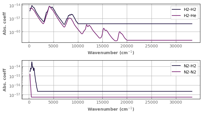
Because CIA are often on very inhomogeneous grids (as above), you will need to sample them on the grid of your Ktable or Xtable to use them.
[74]:
ref_wns_grid=h2o_ktab_SI.wns
cia_data.sample(ref_wns_grid)
fig,axs=plt.subplots(2,1,sharex=False,sharey=False)
cia_data['H2']['H2'].plot_spectrum(axs[0],t=ttest,x_axis='wns',yscale='log',label='H2-H2')
cia_data['H2']['He'].plot_spectrum(axs[0],t=ttest,x_axis='wns',label='H2-He')
cia_data['N2']['H2'].plot_spectrum(axs[1],t=ttest,x_axis='wns',yscale='log',label='N2-H2')
cia_data['N2']['N2'].plot_spectrum(axs[1],t=ttest,x_axis='wns',yscale='log',label='N2-N2')
for ax in axs:
    ax.legend()
fig.tight_layout()
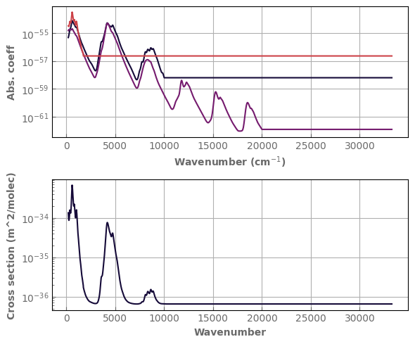
The method:
CIAdatabase.cia_cross_section(pressure,temperature,composition)
can be used to compute the effective CIA cross-section for the whole gas (in m^2 per average molecule)
[75]:
compo={'H2':0.2,'He':0.1,'N2':0.4}
raw=cia_data.cia_cross_section([1.,3.],[300.,500.],compo)
fig,axs=plt.subplots(2,1,sharex=False,sharey=False,figsize=(6,5))
cia_data['H2']['H2'].plot_spectrum(axs[0],t=ttest,x_axis='wns',yscale='log')
cia_data['H2']['He'].plot_spectrum(axs[0],t=ttest,x_axis='wns')
cia_data['N2']['H2'].plot_spectrum(axs[0],t=ttest,x_axis='wns',yscale='log')
axs[1].plot(cia_data.wns,raw[0])
axs[1].set_yscale('log')
axs[1].set_ylabel('Cross section (m^2/molec)')
axs[1].set_xlabel('Wavenumber')
fig.tight_layout()

How to use exo_k as an opacity interpolator inside your code: The Gas_mix object
Exo_k can also be used to directly access and interpolate opacity within your code. For this, one possibility is to load and access individual K/X/CIA tables and add all the opacities by yourself.
Another is to use the Gas_mix object: it contains the information on the pressure/temperature conditions of the gas, its composition, and can be connected to radiative databases to compute the opacity of the gas from all contributions.
Composition and background gas
An empty Gas_mix object can be instanciated as follows and filled later on.
[76]:
gas=xk.Gas_mix()
print(gas)
Volume mixing ratios in Gas_mix:
inactive_gas->1.0
The message shows that, at this time, the Gas_mix is empty. Effectively, it is filled with ‘inactive_gas’.
Composition is specified using a dictionary where molecules are the keys and the volume mixing ratios as values. The rest of the Gas_mix is filled with inactive gas so that Sum(vmr)=1.
[77]:
gas.set_composition({'CO2':0.01})
print(gas)
gas.set_composition({'N2':0.8})  # reset the whole composition
print(gas)
Volume mixing ratios in Gas_mix:
CO2->0.01
inactive_gas->0.99

Volume mixing ratios in Gas_mix:
N2->0.8
inactive_gas->0.19999999999999996
One of the gases can have a vmr equal to ‘background’. In this case, the vmr of this gas will always be updated to be 1.-Sum(other vmrs).
[78]:
gas=xk.Gas_mix({'CO2':0.01,'N2':'background'}) # can also directly instantiate with a composition
print(gas)
gas['O2']=0.2  # only adds a gas or changes its vmr.
print(gas)
gas['H2O']=[0.01, 0.001]  #  Accepts arrays
print(gas)
Volume mixing ratios in Gas_mix:
CO2->0.01
inactive_gas->0.0
N2->0.99

Volume mixing ratios in Gas_mix:
CO2->0.01
inactive_gas->0.0
N2->0.79
O2->0.2

Volume mixing ratios in Gas_mix:
CO2->0.01
inactive_gas->0.0
N2->[0.78  0.789]
O2->0.2
H2O->[0.01  0.001]
Getting the molar mass
The molar mass (in kg/mol) of your mix can be computed simply using:
[79]:
gas.set_composition({'N2':'background','CO2':340.e-6,'H2O':0.001})
print(gas.molar_mass())
gas.set_composition({'CH3COOH':'background'})
print(gas.molar_mass())
gas.set_composition({'Mg3SiO4':'background'})
print(gas.molar_mass())
gas=xk.Gas_mix({'N2':'background','CO2':340.e-6,'H2O':[0.001,0.1]})
print(gas.molar_mass())
0.028008920548799998
0.06005255999999999
0.1649981
[0.02800892 0.0270191 ]
Connecting a gas with a radiative database
To connect with radiative data, first you need to load the databases you want to use. You can combine a CIAdatabase with a Kdatabase filled with either Ktables or Xtables (but not both).
Then these database can be added to a Gas_mix, or you can directly instantiate with these databases. This only needs to be done once.
Warning
With Gas_mix, radiative databases need to be converted in SI units to be used. The simplest way to achieve that is to use exo_k.Settings().set_mks(True).
[80]:
database=xk.Kdatabase(['CO2','H2O'],'R300_0.3-50mu.ktable.SI')

gas.set_k_database(database)

#Loads CIA and sample them on the right spectral grid.
cia_data=xk.CIAdatabase(molecules=['N2','H2O'], mks=True)
cia_data.sample(database.wns)

gas.set_cia_database(cia_data)
print(gas)
Volume mixing ratios in Gas_mix:
CO2->0.00034
H2O->[0.001 0.1  ]
inactive_gas->0.0
N2->[0.99866 0.89966]
Or everything can be done at initialization
[81]:
database=xk.Kdatabase(['CO2','H2O'],'R300_0.3-50mu.ktable.SI')

#Loads CIA and sample them on the right spectral grid.
cia_data=xk.CIAdatabase(molecules=['N2','H2O'], mks=True)
cia_data.sample(database.wns)

gas=xk.Gas_mix(composition={'N2':'background','CO2':340.e-6,'H2O':[0.001,0.1]},
               k_database=database, cia_database=cia_data)
print(gas)
Volume mixing ratios in Gas_mix:
CO2->0.00034
H2O->[0.001 0.1  ]
inactive_gas->0.0
N2->[0.99866 0.89966]
Now, the effective cross section on the gas can be computed as many times as necessary by calling the Gas_mix.cross_section() method providing log pressure (in Pa), temperature, and composition.
[82]:
logp_array=6.
t_array=300.
gas.set_composition({'CO2':0.01,'N2':'background'})
# composition can be set once and for all and only logP and T or changed at call time.
kdata=gas.cross_section(logp_array=logp_array, t_array=t_array)
fig,ax=plt.subplots(1,1,sharey=False,figsize=(8,4))
ax.plot(10000./gas.wns,kdata[0,:,-1])
ax.set_yscale('log')
ax.set_xscale('log')
ax.set_ylabel('Cross section (m^2/molec)')
ax.set_xlabel('Wavelength (micron)')
fig.tight_layout()

[83]:
logp_array=2.
t_array=300.
composition={'N2':'background','CO2':340.e-6,'H2O':1.e-3}
kdata=gas.cross_section(composition=composition, # composition can also be specified at call time
                    logp_array=logp_array, t_array=t_array)

fig,ax=plt.subplots(1,1,sharey=False,figsize=(8,4))
ax.plot(10000./gas.wns,kdata[0,:,-1])
ax.set_yscale('log')
ax.set_xscale('log')
ax.set_ylabel('Cross section (m^2/molec)')
ax.set_xlabel('Wavelength (micron)')
fig.tight_layout()

If you need to call this function for many logP-T points, it is more efficient to call the function once, providing logP-T (and even vmr) arrays
[84]:
logp_array=np.linspace(1.,6.,100)
t_array=300.*np.ones(logp_array.size)
composition={'N2':'background','CO2':340.e-6,
             'H2O':0.001*np.ones(logp_array.size)}
kdata=gas.cross_section(composition=composition,
                    logp_array=logp_array, t_array=t_array)
print(kdata.shape)
(100, 1538, 20)
Choosing gas recombination method (when using Ktables)
Two recombination methods are available when several gases are present:
Simple addition: Fast. It is ok at moderate resolution (and if you are not looking for ppm level accuracy), but can be inacurrate if you are using large bins that encompass molecular bands of several molecules. This is the default mode for
Gas_mix.cross_section().Random overlap: Very accurate in many situations, but a bit longer, especially if you have many molecules. This is the default mode for regular
Ktablerecombinations.
For Gas_mix.cross_section(), the behavior can be controlled with the random_overlap=True/False keyword.
[85]:
logp_array=2.
t_array=300.
gas.set_composition({'N2':'background','CO2':340.e-6,'H2O':0.001})
gas.set_logPT(logp_array=logp_array, t_array=t_array)

kdata=gas.cross_section()
kdata_randoverlap=gas.cross_section(random_overlap=True)

%timeit -r 10 -n 10 gas.cross_section()
%timeit -r 10 -n 10 gas.cross_section(random_overlap=True)


fig,ax=plt.subplots(1,1,sharey=False,figsize=(8,4))
ax.plot(10000./gas.wns,kdata_randoverlap[0,:,-1], label='Rand. Overlap')
ax.plot(10000./gas.wns,kdata[0,:,-1], label='addition')
ax.set_yscale('log')
ax.set_xscale('log')
ax.legend()
ax.set_xlabel('Wavelength (micron)')
ax.set_ylabel('Cross section (m^2/molec)')
fig.tight_layout()
4.09 ms ± 1.15 ms per loop (mean ± std. dev. of 10 runs, 10 loops each)
37.8 ms ± 6.22 ms per loop (mean ± std. dev. of 10 runs, 10 loops each)

You can try any molecule with a regular Element Number of atoms notation.