Some worked out use-cases for exo_k
Author: Jeremy Leconte (CNRS/LAB/Univ. Bordeaux)
Whereas the tutorial goes through all the concepts present in the library in a very progressive manner, here we propose some more complex examples that combine many of these concepts. The idea is to show some ‘real life’ examples of the use of the library that can be adapted by the users to their own needs.
Some of these examples use publicly available data: do not forget to acknowledge them if you use them in your work (see the where to find data section).
General initialization
[1]:
import numpy as np
import matplotlib.pyplot as plt
import astropy.units as u
import time,sys,os
[2]:
# Uncomment the line below if you want to enable interactive plots
#%matplotlib notebook
plt.rcParams["figure.figsize"] = (7,4)
from matplotlib import cycler
font = {'color': 'dimgray', 'weight': 'bold', 'size': 10}
colors = cycler('color',[plt.cm.inferno(i) for i in np.linspace(0.1,1,5)])
plt.rc('axes', axisbelow=True, grid=True, labelcolor='dimgray', labelweight='bold', prop_cycle=colors)
plt.rc('grid', linestyle='solid')
plt.rc('xtick', direction='in', color='dimgray')
plt.rc('ytick', direction='in', color='dimgray')
plt.rc('lines', linewidth=1.5)
Setting up global options for the library
[3]:
import exo_k as xk

datapath='../data/'
#change to your own path

xk.Settings().set_search_path(datapath + 'corrk', path_type='ktable')
xk.Settings().set_search_path(datapath + 'xsec', path_type='xtable')
xk.Settings().set_search_path(datapath + 'cia', path_type='cia')

xk.Settings().set_mks(True)
# to automatically convert to mks units
Loading ExoMol files and changing their resolution before saving them in different formats
For this, you will need to download the relevant x-sec of ktable files from the ExoMol website http://exomol.com/data/data-types/opacity/ into the datapath/xsec or datapath/corrk.
[4]:
#let's decide on the spectral grid we want:
wn0=200.
wn1=10000.
Resolution=20.
new_wn_grid=xk.wavenumber_grid_R(wn0, wn1, Resolution)
# Here it is a grid a constant resolution, but any numpy array will do.

# a more focused logP-T grid
logp_array=np.arange(8)
t_array=np.arange(100,600,100)

dir_out=datapath + 'corrk/'

molecules = ['1H2-16O','12C-16O2','12C-1H4']
for mol in molecules:
    tmp_ktab=xk.Ktable(mol,'R1000_0.3-50mu.ktable.petitRADTRANS.h5', remove_zeros=True)

    # if for some reasons you need to limit the P-T grid (optional)
    tmp_ktab.remap_logPT(logp_array=logp_array, t_array=t_array)

    # the spectral binning phase
    tmp_ktab.bin_down(new_wn_grid)
    print(tmp_ktab)
    # choose any of the lines below for different formats
    tmp_ktab.write_hdf5(dir_out+mol+'_R20.ktable') # hdf5 file with current units
    #tmp_ktab.write_hdf5(dir_out+mol+'_R20.ktable', exomol_units=True) # hdf5 file with Exomol units
    #tmp_ktab.write_nemesis(dir_out+mol+'_R20.ktable') # binary nemesis format
    #tmp_ktab.write_arcis(dir_out+mol+'_R20.ktable') # fits ARCIS format
        file         : /builds/jleconte/exo_k-public/data/corrk/1H2-16O__POKAZATEL__R1000_0.3-50mu.ktable.petitRADTRANS.h5
        molecule     : 1H2-16O
        p grid       : [1.e+00 1.e+01 1.e+02 1.e+03 1.e+04 1.e+05 1.e+06 1.e+07]
        p unit       : Pa
        t grid   (K) : [100 200 300 400 500]
        wn grid      : [ 205.12710964  215.64420145  226.70051608  238.32370009  250.54281748
  263.38842243  276.89263562  291.08922462  306.01368831  321.70334562
  338.19742886  355.53718183  373.76596294  392.92935365  413.07527241
  434.25409451  456.51877804  479.92499631  504.53127705  530.39914878
  557.59329465  586.1817142   616.23589336  647.83098324  681.04598802
  715.96396251  752.67221983  791.26254975  831.8314482   874.48035855
  919.31592529  966.4502607  1016.00122516 1068.09272189 1122.85500677
 1180.42501404 1240.9466987  1304.57139649 1371.45820229 1441.77436795
 1515.69572052 1593.40710189 1675.10283097 1760.98718966 1851.27493358
 1946.19182912 2045.97521795 2150.87461054 2261.15230999 2377.08406799
 2498.95977434 2627.08418177 2761.77766804 2903.37703702 3052.23636091
 3208.72786553 3373.24286117 3546.192721   3728.00990977 3919.14906514
 4120.08813457 4331.3295704  4553.40158624 4786.85947781 5032.28701143
 5290.29788379 5561.53725644 5846.68336912 6146.44923561 6461.58442674
 6792.87694463 7141.15519313 7507.29004927 7892.19704091 8296.83863601
 8722.22664934 9169.42477249 9639.55123371 9940.24491055]
        wn unit      : cm^-1
        kdata unit   : m^2/molecule
        weights      : [0.04555284 0.10007147 0.14116799 0.1632077  0.1632077  0.14116799
 0.10007147 0.04555284 0.00506143 0.01111905 0.01568533 0.01813419
 0.01813419 0.01568533 0.01111905 0.00506143]
        data oredered following p, t, wn, g
        shape        : [ 8  5 79 16]


        file         : /builds/jleconte/exo_k-public/data/corrk/12C-16O2__UCL-4000.R1000_0.3-50mu.ktable.petitRADTRANS.h5
        molecule     : CO2
        p grid       : [1.e+00 1.e+01 1.e+02 1.e+03 1.e+04 1.e+05 1.e+06 1.e+07]
        p unit       : Pa
        t grid   (K) : [100 200 300 400 500]
        wn grid      : [ 205.12710964  215.64420145  226.70051608  238.32370009  250.54281748
  263.38842243  276.89263562  291.08922462  306.01368831  321.70334562
  338.19742886  355.53718183  373.76596294  392.92935365  413.07527241
  434.25409451  456.51877804  479.92499631  504.53127705  530.39914878
  557.59329465  586.1817142   616.23589336  647.83098324  681.04598802
  715.96396251  752.67221983  791.26254975  831.8314482   874.48035855
  919.31592529  966.4502607  1016.00122516 1068.09272189 1122.85500677
 1180.42501404 1240.9466987  1304.57139649 1371.45820229 1441.77436795
 1515.69572052 1593.40710189 1675.10283097 1760.98718966 1851.27493358
 1946.19182912 2045.97521795 2150.87461054 2261.15230999 2377.08406799
 2498.95977434 2627.08418177 2761.77766804 2903.37703702 3052.23636091
 3208.72786553 3373.24286117 3546.192721   3728.00990977 3919.14906514
 4120.08813457 4331.3295704  4553.40158624 4786.85947781 5032.28701143
 5290.29788379 5561.53725644 5846.68336912 6146.44923561 6461.58442674
 6792.87694463 7141.15519313 7507.29004927 7892.19704091 8296.83863601
 8722.22664934 9169.42477249 9639.55123371 9940.24491055]
        wn unit      : cm^-1
        kdata unit   : m^2/molecule
        weights      : [0.04555284 0.10007147 0.14116799 0.1632077  0.1632077  0.14116799
 0.10007147 0.04555284 0.00506143 0.01111905 0.01568533 0.01813419
 0.01813419 0.01568533 0.01111905 0.00506143]
        data oredered following p, t, wn, g
        shape        : [ 8  5 79 16]


        file         : /builds/jleconte/exo_k-public/data/corrk/12C-1H4__YT34to10.R1000_0.3-50mu.ktable.petitRADTRANS.h5
        molecule     : CH4
        p grid       : [1.e+00 1.e+01 1.e+02 1.e+03 1.e+04 1.e+05 1.e+06 1.e+07]
        p unit       : Pa
        t grid   (K) : [100 200 300 400 500]
        wn grid      : [ 205.12710964  215.64420145  226.70051608  238.32370009  250.54281748
  263.38842243  276.89263562  291.08922462  306.01368831  321.70334562
  338.19742886  355.53718183  373.76596294  392.92935365  413.07527241
  434.25409451  456.51877804  479.92499631  504.53127705  530.39914878
  557.59329465  586.1817142   616.23589336  647.83098324  681.04598802
  715.96396251  752.67221983  791.26254975  831.8314482   874.48035855
  919.31592529  966.4502607  1016.00122516 1068.09272189 1122.85500677
 1180.42501404 1240.9466987  1304.57139649 1371.45820229 1441.77436795
 1515.69572052 1593.40710189 1675.10283097 1760.98718966 1851.27493358
 1946.19182912 2045.97521795 2150.87461054 2261.15230999 2377.08406799
 2498.95977434 2627.08418177 2761.77766804 2903.37703702 3052.23636091
 3208.72786553 3373.24286117 3546.192721   3728.00990977 3919.14906514
 4120.08813457 4331.3295704  4553.40158624 4786.85947781 5032.28701143
 5290.29788379 5561.53725644 5846.68336912 6146.44923561 6461.58442674
 6792.87694463 7141.15519313 7507.29004927 7892.19704091 8296.83863601
 8722.22664934 9169.42477249 9639.55123371 9940.24491055]
        wn unit      : cm^-1
        kdata unit   : m^2/molecule
        weights      : [0.04555284 0.10007147 0.14116799 0.1632077  0.1632077  0.14116799
 0.10007147 0.04555284 0.00506143 0.01111905 0.01568533 0.01813419
 0.01813419 0.01568533 0.01111905 0.00506143]
        data oredered following p, t, wn, g
        shape        : [ 8  5 79 16]
Creating k-coefficients for a new species not in ExoMol from high-resolution spectra from the petitRADTRANS database
Start by downloading some high resolution cross sections from petitRADTRANS: https://www.dropbox.com/sh/w7sa20v8qp19b4d/AABKF0GsjghsYLJMUJXDgrHma?dl=0
Here I am using data for Na. For the example to work with as few data as possible, I only consider a grid with 2 P and T points. So you will only need the following files in the Na directory:
‘sigma_94_1215.K_0.001000bar.dat’
‘sigma_94_1641.K_0.001000bar.dat’
‘sigma_94_1215.K_1.000000bar.dat’
‘sigma_94_1641.K_1.000000bar.dat’
wlen.dat
Feel free to extend to the full grid once you have downloaded the whole dataset.
[5]:
path_to_hires_spectra=datapath + 'hires/PetitRADTRANS/Na'

press_grid_str=['0.001000','1.000000']  # notice the use of strings
logp_grid=[np.log10(float(p)) for p in press_grid_str]
t_grid=[1215, 1641]

file_grid=xk.create_fname_grid('sigma_94_{temp}.K_{press}bar.dat', logpgrid=press_grid_str, tgrid=t_grid,
        p_kw='press', t_kw='temp')
print(file_grid)

Hires_spectra=xk.hires_to_xtable(path=path_to_hires_spectra, filename_grid=file_grid, logpgrid=logp_grid, tgrid=t_grid,
                mol='Na', grid_p_unit='bar', binary=True, mass_amu=23.)

Hires_spectra
[['sigma_94_1215.K_0.001000bar.dat' 'sigma_94_1641.K_0.001000bar.dat']
 ['sigma_94_1215.K_1.000000bar.dat' 'sigma_94_1641.K_1.000000bar.dat']]
[5]:
        file         : ../data/hires/PetitRADTRANS/Na
        molecule     : Na
        p grid       : [   100. 100000.]
        p unit       : Pa
        t grid   (K) : [1215 1641]
        wn grid      : [  357.14265128   357.14300842   357.14336556 ... 33333.23696353
 33333.27029679 33333.30363008]
        wn unit      : cm^-1
        kdata unit   : m^2/molecule
        data oredered following p, t, wn
        shape        : [      2       2 4536178]
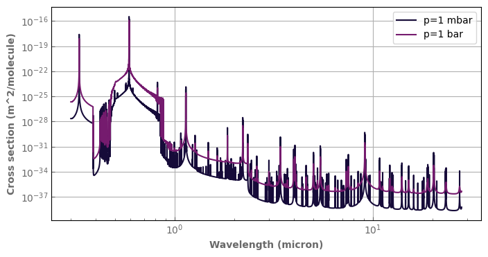
[6]:
fig,ax=plt.subplots(1,1,sharey=False, figsize=(8,4))
Hires_spectra.plot_spectrum(ax, p=1.e3, t=1300., xscale='log', yscale='log', label='p=1 mbar')
Hires_spectra.plot_spectrum(ax, p=1.e5, t=1300., label='p=1 bar')
ax.legend(loc='upper right')
plt.show()
[7]:
# Let's load a conventional ExoMOL k-table to use the same wavenumber and
#    g-grid
tmp_ktab=xk.Ktable('1H2-16O','R1000_0.3-50mu.ktable.petitRADTRANS.h5', remove_zeros=True)

wnedges=tmp_ktab.wnedges
weights=tmp_ktab.weights
ggrid=tmp_ktab.ggrid
## Or we can create a custom g-grid with 8 gauss legendre points between 0 and 0.95
##   and 8 points between 0.95 and 1 (as usual with petitRADTRANS data)
#weights, ggrid, gedges = xk.split_gauss_legendre(order=16, g_split=0.95)

ktab=xk.Ktable(xtable=Hires_spectra, wnedges=wnedges, weights=weights, ggrid=ggrid, remove_zeros=True)

## choose any of the lines below for different formats
#full_path_to_write=datapath + 'corrk/Na_R1000.ktable'
#tmp_ktab.write_hdf5(full_path_to_write) # hdf5 file with current units
#tmp_ktab.write_hdf5(full_path_to_write, exomol_units=True) # hdf5 file with Exomol units
#tmp_ktab.write_nemesis(full_path_to_write) # binary nemesis format
#tmp_ktab.write_arcis(full_path_to_write) # fits ARCIS format
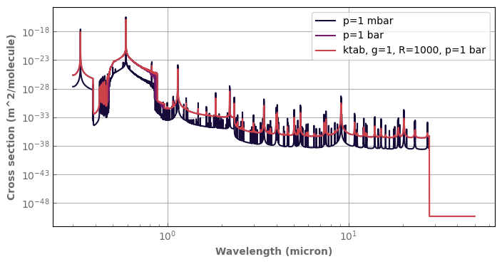
[8]:
fig,ax=plt.subplots(1,1,sharey=False, figsize=(8,4))
Hires_spectra.plot_spectrum(ax, p=1.e3, t=1300., xscale='log', yscale='log', label='p=1 mbar')
Hires_spectra.plot_spectrum(ax, p=1.e5, t=1300., label='p=1 bar')
ktab.plot_spectrum(ax, p=1.e5, t=1300., g=1, label='ktab, g=1, R=1000, p=1 bar')
ax.legend(loc='upper right')
plt.show()
Modelling transit spectra: sampled cross sections vs. k-coefficients (Leconte, A&A, 2020)
Here we will reproduce some of the results shown in Leconte (A&A, 2020) that demonstrate that the correlated-k method can be much more accurate than the sampled cross-section technique in many cases of interest. Although we use a different set of initial data (because these are publicly available and easily accessible), the results are mostly unaffected.
Start by downloading some high resolution cross sections for water from petitRADTRANS: https://www.dropbox.com/sh/w7sa20v8qp19b4d/AABKF0GsjghsYLJMUJXDgrHma?dl=0
[9]:
path_to_hires_spectra=datapath + 'hires/PetitRADTRANS/H2O/'

press_grid_str=['0.000001','0.000010','0.000100','0.001000','0.010000','0.100000','1.000000','10.000000','100.000000']
logp_grid=[np.log10(float(p)) for p in press_grid_str]
t_grid=[900, 1215]

file_grid=xk.create_fname_grid('sigma_01_{temp}.K_{press}bar.dat', logpgrid=press_grid_str, tgrid=t_grid,
        p_kw='press', t_kw='temp')
print(file_grid)

h2o_hires=xk.hires_to_xtable(path=path_to_hires_spectra, filename_grid=file_grid, logpgrid=logp_grid, tgrid=t_grid,
                mol='H2O', grid_p_unit='bar', binary=True, mass_amu=18.)

h2o_hires
[['sigma_01_900.K_0.000001bar.dat' 'sigma_01_1215.K_0.000001bar.dat']
 ['sigma_01_900.K_0.000010bar.dat' 'sigma_01_1215.K_0.000010bar.dat']
 ['sigma_01_900.K_0.000100bar.dat' 'sigma_01_1215.K_0.000100bar.dat']
 ['sigma_01_900.K_0.001000bar.dat' 'sigma_01_1215.K_0.001000bar.dat']
 ['sigma_01_900.K_0.010000bar.dat' 'sigma_01_1215.K_0.010000bar.dat']
 ['sigma_01_900.K_0.100000bar.dat' 'sigma_01_1215.K_0.100000bar.dat']
 ['sigma_01_900.K_1.000000bar.dat' 'sigma_01_1215.K_1.000000bar.dat']
 ['sigma_01_900.K_10.000000bar.dat' 'sigma_01_1215.K_10.000000bar.dat']
 ['sigma_01_900.K_100.000000bar.dat' 'sigma_01_1215.K_100.000000bar.dat']]
[9]:
        file         : ../data/hires/PetitRADTRANS/H2O/
        molecule     : H2O
        p grid       : [1.e-01 1.e+00 1.e+01 1.e+02 1.e+03 1.e+04 1.e+05 1.e+06 1.e+07]
        p unit       : Pa
        t grid   (K) : [ 900 1215]
        wn grid      : [  357.14265128   357.14300842   357.14336556 ... 33333.23696353
 33333.27029679 33333.30363008]
        wn unit      : cm^-1
        kdata unit   : m^2/molecule
        data oredered following p, t, wn
        shape        : [      9       2 4536178]
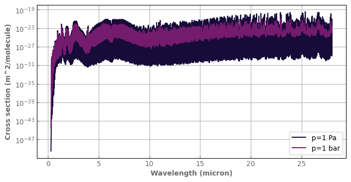
Notice the pressure grid has been automatically converted to Pa
[10]:
fig,ax=plt.subplots(1,1,sharey=False, figsize=(8,4))
h2o_hires.plot_spectrum(ax, p=1., t=1000., yscale='log', label='p=1 Pa')
h2o_hires.plot_spectrum(ax, p=1.e5, t=1000., yscale='log', label='p=1 bar')
ax.legend(loc='lower right')
plt.show()
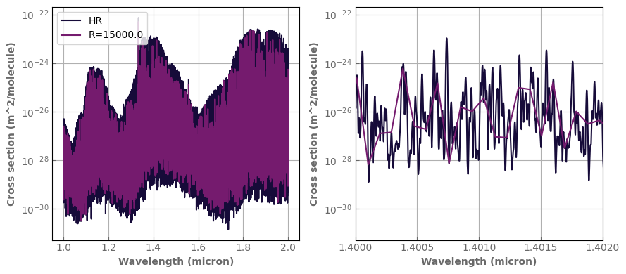
We clip the data to focus on a smaller wavenumber range (roughly, the WFC3 region).
[11]:
wn0=5000.
wn1=10000.

h2o_hires.clip_spectral_range(wn_range=[wn0-2.,wn1+2.])
[12]:
Ri=15000.
wn_interm_grid=xk.wavenumber_grid_R(wn0, wn1, Ri)
sampled=h2o_hires.sample_cp(wn_interm_grid)

fig,axs=plt.subplots(1,2,sharey=False, figsize=(9,4))
h2o_hires.plot_spectrum(axs[0], p=1., t=1000., yscale='log', label='HR')
sampled.plot_spectrum(axs[0], p=1., t=1000., yscale='log', label='R='+str(Ri))
h2o_hires.plot_spectrum(axs[1], p=1., t=1000., yscale='log', label='HR')
sampled.plot_spectrum(axs[1], p=1., t=1000., yscale='log', label='R='+str(Ri))
axs[0].legend(loc='upper left')
axs[1].set_xlim(1.4,1.402)
fig.tight_layout()
I can directly write this to an hdf5 file that is compatible with TauREX and petitRADTRANS (see above)
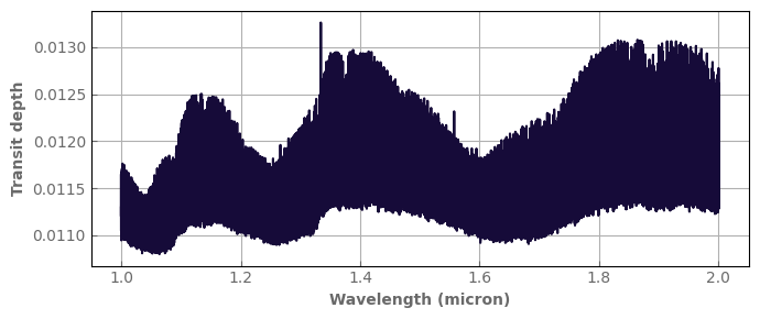
Now let’s compute a reference, high-resolution transmission spectrum:
[13]:
start=time.time()

database=xk.Kdatabase(None)
database.add_ktables(h2o_hires)

T0=1000.; xH2O=1.e-3; Rp=1*u.Rjup; Rs=1.*u.Rsun; grav=10.; nlay=100;

atm=xk.Atm(psurf=10.e5, ptop=1.e-4, Tsurf=T0, grav=grav, rcp=0.28,
                    composition={'H2':'background','H2O':xH2O}, Nlay=nlay, Rp=Rp,
                    k_database=database)
spec_ref=atm.transmission_spectrum(Rstar=Rs)

print('computation time=',time.time()-start,'s')
computation time= 14.453312635421753 s
[14]:
fig,ax=plt.subplots(1,1,sharex=True,figsize=(7,3))
spec_ref.plot_spectrum(ax)
ax.set_ylabel('Transit depth', fontdict=font)
fig.tight_layout()
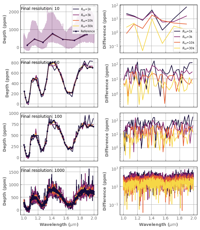
In the following, we sample our cross sections on a grid of intermediate resolution (Rinter) to compute the spectrum and then bin down to the desired final resolution
[15]:
timeit=False
#grid of final (instrumental data) resolution
Rfin=[10,20,50,100.,200.,500.,1000.]
#grid of intermediate resolution (at which computation will be performed)
Rinter=[1000.,3000.,10000.,30000.]

start=time.time()
res=[]
for Ri in Rinter:
    wn_interm_grid=xk.wavenumber_grid_R(wn0, wn1, Ri)
    database_LR=database.copy()
    database_LR.sample(wn_interm_grid)
    atm.set_k_database(k_database=database_LR)
    spec_LR=atm.transmission_spectrum(Rstar=Rs)
    if timeit:
        %timeit atm.transmission_spectrum(Rstar=Rs)
    for Rf in Rfin:
        print('intermediate resolution=',Ri,', final resolution=',Rf)
        wn_final_grid=xk.wavenumber_grid_R(wn0, wn1, Rf)
        spectmp=spec_LR.bin_down_cp(wn_final_grid)
        spec_comp=spec_ref.bin_down_cp(wn_final_grid)
        res.append([Ri,Rf,(spectmp-spec_comp).std(),spectmp,spectmp-spec_comp])

print('computation time=',time.time()-start,'s')
res2=np.array(res).reshape((len(Rinter),len(Rfin),5))
intermediate resolution= 1000.0 , final resolution= 10
intermediate resolution= 1000.0 , final resolution= 20
intermediate resolution= 1000.0 , final resolution= 50
intermediate resolution= 1000.0 , final resolution= 100.0
intermediate resolution= 1000.0 , final resolution= 200.0
intermediate resolution= 1000.0 , final resolution= 500.0
intermediate resolution= 1000.0 , final resolution= 1000.0
intermediate resolution= 3000.0 , final resolution= 10
intermediate resolution= 3000.0 , final resolution= 20
intermediate resolution= 3000.0 , final resolution= 50
intermediate resolution= 3000.0 , final resolution= 100.0
intermediate resolution= 3000.0 , final resolution= 200.0
intermediate resolution= 3000.0 , final resolution= 500.0
intermediate resolution= 3000.0 , final resolution= 1000.0
intermediate resolution= 10000.0 , final resolution= 10
intermediate resolution= 10000.0 , final resolution= 20
intermediate resolution= 10000.0 , final resolution= 50
intermediate resolution= 10000.0 , final resolution= 100.0
intermediate resolution= 10000.0 , final resolution= 200.0
intermediate resolution= 10000.0 , final resolution= 500.0
intermediate resolution= 10000.0 , final resolution= 1000.0
intermediate resolution= 30000.0 , final resolution= 10
intermediate resolution= 30000.0 , final resolution= 20
intermediate resolution= 30000.0 , final resolution= 50
intermediate resolution= 30000.0 , final resolution= 100.0
intermediate resolution= 30000.0 , final resolution= 200.0
intermediate resolution= 30000.0 , final resolution= 500.0
intermediate resolution= 30000.0 , final resolution= 1000.0
computation time= 1.2983903884887695 s
Here are the spectra for each intermediate and final resolution. The right column shows the difference with the reference, high-resolution spectrum.
[16]:
to_plot=res2[:,[0,2,3,6]]
nRfin=to_plot.shape[1]
fig,axs=plt.subplots(nRfin,2,sharex=True,figsize=(7,8))
color_idx = np.linspace(0.1, 0.9, to_plot.shape[0])
offset=11000.
for iRfin in range(nRfin):
    for i, data in enumerate(to_plot[:,iRfin]):
        (data[3]*1.e6-offset).plot_spectrum(axs[iRfin,0],label='$R_{sp}$='+str(int(data[0]/1.e3))+'k',
                    color=plt.cm.inferno(color_idx[i]))
        (data[4].abs()*1.e6).plot_spectrum(axs[iRfin,1],yscale='log',
                    label='$R_{sp}$='+str(int(data[0]/1.e3))+'k',
                    color=plt.cm.inferno(color_idx[i]))
    wn_final_grid=xk.wavenumber_grid_R(wn0,wn1,to_plot[0,iRfin,1])
    spec_comp=spec_ref.bin_down_cp(wn_final_grid)
    (spec_comp*1.e6-offset).plot_spectrum(axs[iRfin,0],marker='.', label='Reference')
    if iRfin==0:
        (spec_ref*1.e6-offset).plot_spectrum(axs[0,0],alpha=0.3)
        axs[iRfin,0].legend(fontsize='x-small', loc='upper right')
        axs[iRfin,1].legend(fontsize='x-small')
    axs[iRfin,0].text(0.01, .9, 'Final resolution: '+str(int(to_plot[0,iRfin,1])), transform=axs[iRfin,0].transAxes)
    axs[iRfin,0].set_ylabel('Depth (ppm)', fontdict=font)
    axs[iRfin,1].set_ylabel('Difference (ppm)', fontdict=font)
    axs[iRfin,0].set_xlabel(None)
    axs[iRfin,1].set_xlabel(None)
axs[-1,0].set_xlabel(r'Wavelength ($\mu m$)', fontdict=font)
axs[-1,1].set_xlabel(r'Wavelength ($\mu m$)', fontdict=font)
fig.tight_layout()
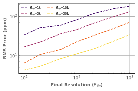
Let’s summarize these results by looking only at the RMS error as a function of the final resolution for various intermediate resolutions.
[17]:
nRint=res2.shape[0]
color_idx = np.linspace(0.2, 0.9, nRint)
fig,ax=plt.subplots(1,1, sharex=True, figsize= (4.5,3))
for iRint in range(nRint):
    ax.plot(res2[iRint,:,1], res2[iRint,:,2]*1.e6, label='$R_{sp}$='+str(int(res2[iRint,0,0]/1.e3))+'k',
            color=plt.cm.inferno(color_idx[iRint]), linestyle='--')
ax.set_xscale('log')
ax.set_yscale('log')
ax.set_ylabel('RMS Error (ppm)', fontdict=font)
ax.set_xlabel('Final Resolution ($R_{fin}$)', fontdict=font)
ax.legend(fontsize='x-small', loc="upper left", ncol=2, frameon=False)
fig.tight_layout()
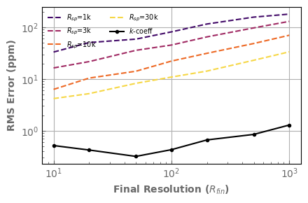
Finaly, let’s compare with the result given by the correlated-k approach, computed directly at the final resolution.
[18]:
rescorrk=[]
order=8
for Rf in Rfin:
    print('Resolution=', Rf)
    wn_final_grid=xk.wavenumber_grid_R(wn0, wn1, Rf)
    database_corrk=xk.Kdatabase(None)
    database_corrk.add_ktables(xk.Ktable(xtable=h2o_hires, wnedges=wn_final_grid, order=order))
    atm.set_k_database(k_database=database_corrk)
    spec_corrk=atm.transmission_spectrum(Rstar=Rs)
    if timeit:
        %timeit atm.transmission_spectrum(Rstar=Rs)
    spectmp=spec_corrk.copy()
    spec_comp=spec_ref.bin_down_cp(wn_final_grid)
    rescorrk.append([1.,Rf,(spectmp-spec_comp).std(),spectmp,spectmp-spec_comp])

rescorrk=np.array(rescorrk).reshape((len(Rfin),5))
Resolution= 10
Resolution= 20
Resolution= 50
Resolution= 100.0
Resolution= 200.0
Resolution= 500.0
Resolution= 1000.0
[19]:
nRint=res2.shape[0]
color_idx = np.linspace(0.2, 0.9, nRint)
fig,ax=plt.subplots(1,1, sharex=True, figsize= (4.5,3))
for iRint in range(nRint):
    ax.plot(res2[iRint,:,1], res2[iRint,:,2]*1.e6, label='$R_{sp}$='+str(int(res2[iRint,0,0]/1.e3))+'k',
            color=plt.cm.inferno(color_idx[iRint]), linestyle='--')
ax.plot(rescorrk[:,1], rescorrk[:,2]*1.e6, marker='.', color='k', label='$k$-coeff')
ax.set_xscale('log')
ax.set_yscale('log')
ax.set_ylabel('RMS Error (ppm)', fontdict=font)
ax.set_xlabel('Final Resolution ($R_{fin}$)', fontdict=font)
ax.legend(fontsize='x-small', loc="upper left", ncol=2, frameon=False)
fig.tight_layout()
Create spectra on a different wavelength region
[20]:
path_to_hires_spectra=datapath + 'hires/PetitRADTRANS/H2O/'

press_grid_str=['0.000001','0.000010','0.000100','0.001000','0.010000','0.100000','1.000000','10.000000','100.000000']
logp_grid=[np.log10(float(p)) for p in press_grid_str]
t_grid=[900, 1215]

wn0=1000.
wn1=20000.

Ri=1000.
wn_interm_grid=xk.wavenumber_grid_R(wn0, wn1, Ri)

file_grid=xk.create_fname_grid('sigma_01_{temp}.K_{press}bar.dat', logpgrid=press_grid_str, tgrid=t_grid,
        p_kw='press', t_kw='temp')
print(file_grid)

h2o_ktab=xk.hires_to_ktable(path=path_to_hires_spectra, wnedges=wn_interm_grid, filename_grid=file_grid, logpgrid=logp_grid, tgrid=t_grid,
                mol='H2O', grid_p_unit='bar', binary=True, mass_amu=18.)

h2o_ktab
[['sigma_01_900.K_0.000001bar.dat' 'sigma_01_1215.K_0.000001bar.dat']
 ['sigma_01_900.K_0.000010bar.dat' 'sigma_01_1215.K_0.000010bar.dat']
 ['sigma_01_900.K_0.000100bar.dat' 'sigma_01_1215.K_0.000100bar.dat']
 ['sigma_01_900.K_0.001000bar.dat' 'sigma_01_1215.K_0.001000bar.dat']
 ['sigma_01_900.K_0.010000bar.dat' 'sigma_01_1215.K_0.010000bar.dat']
 ['sigma_01_900.K_0.100000bar.dat' 'sigma_01_1215.K_0.100000bar.dat']
 ['sigma_01_900.K_1.000000bar.dat' 'sigma_01_1215.K_1.000000bar.dat']
 ['sigma_01_900.K_10.000000bar.dat' 'sigma_01_1215.K_10.000000bar.dat']
 ['sigma_01_900.K_100.000000bar.dat' 'sigma_01_1215.K_100.000000bar.dat']]
[20]:
        file         : ../data/hires/PetitRADTRANS/H2O/
        molecule     : H2O
        p grid       : [1.e-01 1.e+00 1.e+01 1.e+02 1.e+03 1.e+04 1.e+05 1.e+06 1.e+07]
        p unit       : Pa
        t grid   (K) : [ 900 1215]
        wn grid      : [ 1000.50025008  1001.50125075  1002.50325292 ... 19955.40681676
 19975.37220461 19992.67994494]
        wn unit      : cm^-1
        kdata unit   : m^2/molecule
        weights      : [0.008807   0.02030071 0.03133602 0.04163837 0.05096506 0.05909727
 0.06584432 0.07104805 0.07458649 0.07637669 0.07637669 0.07458649
 0.07104805 0.06584432 0.05909727 0.05096506 0.04163837 0.03133602
 0.02030071 0.008807  ]
        data oredered following p, t, wn, g
        shape        : [   9    2 2996   20]
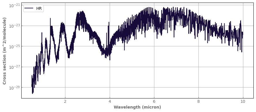
[21]:
fig,ax=plt.subplots(1,1,sharey=False, figsize=(9,4))
h2o_ktab.plot_spectrum(ax, p=1., t=1000., g=1., yscale='log', label='HR')
ax.legend(loc='upper left')
fig.tight_layout()
plt.show()
[22]:
start=time.time()

database=xk.Kdatabase(None)
database.add_ktables(h2o_ktab)

T0=1000.; xH2O=1.e-3; Rp=1*u.Rjup; Rs=1.*u.Rsun; grav=10.; nlay=100;

atm=xk.Atm(psurf=10.e5, ptop=1.e-4, Tsurf=T0, grav=grav, rcp=0.28,
                    composition={'H2':'background','H2O':xH2O}, Nlay=nlay, Rp=Rp,
                    k_database=database)
spec_ref=atm.transmission_spectrum(Rstar=Rs, rayleigh=True)

print('computation time=',time.time()-start,'s')
computation time= 0.5757811069488525 s
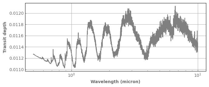
[23]:
wn0=5000.
wn1=20000.

Rlow=25.
wn_lowres=xk.wavenumber_grid_R(wn0, wn1, Rlow)

fig,ax=plt.subplots(1,1,sharex=True,figsize=(7,3))
spec_ref.plot_spectrum(ax, color='gray', xscale='log')
#spec_ref.bin_down_cp(wnedges=wn_lowres).plot_spectrum(ax, marker='.', color='gray')
ax.set_ylabel('Transit depth', fontdict=font)
fig.tight_layout()
# plt.savefig('Spectrum.pdf')