General configuration
User-specific paths to cross-section, CIA, and aerosols data files
First, you need to configure the paths where cross-section, CIA, and aerosols data files are located. xsec_path may indicate either cross-sections or correlated-k data.
If you want to test this tutorial notebook, you can download simple example data at https://mycore.core-cloud.net/index.php/s/w2cHuigAiwcfBVW. To download and move the data in the correct paths, you can uncomment the following cell:
[1]:
# ! wget https://forge.oasu.u-bordeaux.fr/amechineau/pytmosph3r-data/-/archive/minimal/pytmosph3r-data-minimal.zip
# ! unzip pytmosph3r-data-minimal.zip
# ! mkdir -p data
# ! mv pytmosph3r-data-minimal/* data/   # or if you already have data/, update it with: rsync -avz exo_k-public/ data/
# ! ln -sf data/gcm/K2-18b_diagfi.nc diagfi.nc    # try either this one (with aerosols) ...
# ! ln -sf data/gcm/wasp121b_Teq2100.nc diagfi.nc # ... or this one (Ultra Hot Jupiter)
Many thanks to [ParmentierLineBean+18] and [CharnayBlainBezard+21] for providing the simulations available in this example.
[2]:
from pathlib import Path

# Path where the data are stored
data_path: Path = Path('..') / 'data'

xsec_path = (data_path / "corrk").as_posix()
aerosol_path = (data_path / "aerosol").as_posix()
cia_path = (data_path / "cia").as_posix()
General Imports
Now let’s import some general libraries and set the paths that we’ve just configured for Pytmosph3R.
[3]:
import numpy as np

import astropy.units as u
import pytmosph3r as p3
import exo_k as xk

p3.criticalLogging() # disable most of the logging
xk.Settings().set_search_path(xsec_path)
xk.Settings().set_cia_search_path(cia_path)
xk.Settings().set_aerosol_search_path(aerosol_path)

#xk.Settings().set_delimiter(".")
xk.Settings().set_mks(True)
xk.Settings().set_log_interp(False)

# %matplotlib notebook
In case you encounter a bug, you can use the following command to get more information from pytmosph3r:
[4]:
p3.debug()
And return to the default behavior:
[5]:
p3.debug(False)
Simple transmission model configuration
We can now setup our Pytmosph3R model! This can be done with an input file (see library_input), or by constructing a simple atmosphere, as shown below.
Planet & star
Let’s configure a planet and a star to put in our model, we suppose a tidal locked orbit with a radius of 1 AU:
[6]:
Rp = 1.807 * 6.9911e7 * u.Unit('m')
g0 = 6.67384e-11 * 1.183 * 1.898e27 / Rp**2 * u.Unit('m3*s-2')

orbit=p3.CircularOrbit(a=1.*u.au)
planet = p3.Planet(surface_gravity=g0, radius=Rp)
star = p3.Star.fromSolar(temperature=6460.0, radius=1.458) # radius is in sun radii
Atmosphere
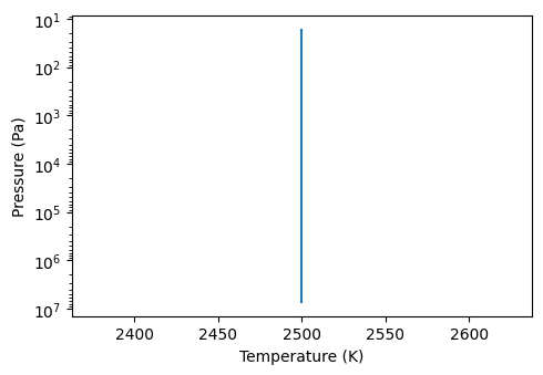
First, let’s choose the dimensions of our atmospheric grid. Here, we will first test a 1D model:
[7]:
grid = p3.Grid3D(n_vertical=100, n_latitudes=1, n_longitudes=1)
We can now set the temperature, pressure and gases to include in our atmosphere:
[8]:
input_atmosphere = p3.InputAtmosphere(grid=grid,

     # Feel free to add a 1D temperature profile here instead
     temperature = 2500,

     # bottom and top pressures
     max_pressure = 1e6, min_pressure = 1e-4,

     # Again, you could add more complex molecular profiles if needed
     gas_mix_ratio = {"H2O":5.01187234e-04,
                      "CO2":4.4e-4,
                      "H2":"background"
                     },
     # molecules for which we will not compute the opacity
     transparent_gases = "H2")
To choose the position of the observer and the number of rays, you can use:
[9]:
observer = p3.Observer(0, 180) # latitude, longitude in degrees
rays = p3.Rays(n_radial=100, n_angular=1) # in 1D cases, only 1 angle is required
Opacity
Let’s choose what kind of opacity we want to put in there:
[10]:
opacity = p3.Opacity(rayleigh=True, cia=['H2', 'He'])
Run the model
The model can be initialized using:
[11]:
model = p3.Model(n_vertical = 100,
                 planet=planet,
                 star=star,
                 orbit=orbit,
                 observer=observer,
                 input_atmosphere=input_atmosphere,
                 transmission=p3.Transmission(rays=rays),
                 opacity=opacity,)

model.build()
And now you can run it with:
[12]:
model.run()
be careful: ()
            String filters not specific enough, several corresponding files have been found.
            We will use the first one:
            /builds/jleconte/pytmosph3r-public/data/corrk/H2O_R300_0.3-50mu.ktable.SI.h5
            Other files are:
            ['/builds/jleconte/pytmosph3r-public/data/corrk/H2O_R300_0.3-50mu.ktable.TauREx.h5']
Variables in the model
If you need more information about an object, you can checkout its inputs and outputs by just calling it:
[13]:
model
[13]:
 Model()
- Inputs: ['output_file', 'n_vertical', 'noise', 'interp', 'gas_dict', 'aerosols_dict', 'input_atmosphere', 'opacity', 'planet', 'star', 'observer', 'orbit', 'radiative_transfer', 'transmission', 'emission', 'lightcurve', 'phasecurve', 'parallel']
- Outputs: ['input_atmosphere', 'atmosphere', 'wns', 'wnedges', 'transmission', 'emission', 'lightcurve', 'phasecurve', 'spectrum_value', 'spectrum_noised']
- Methods: ['Rp', 'aerosol', 'available_memory', 'build', 'check_memory', 'critical', 'debug', 'default_value', 'dump_profiling', 'error', 'gas', 'info', 'inputs', 'inputs_values', 'isEnabledFor', 'outputs', 'override_data_file', 'override_file_param', 'read_data', 'run', 'search_path', 'start_profiling', 'summary', 'warning']
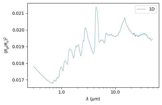
Plot the spectrum
The spectrum can be visualized with:
[14]:
plot = p3.Plot(model=model, label="1D", interactive=True, out_folder="outputs")
plot.plot_spectrum()
Saved to `outputs/spectrum_pytmosph3r.pdf`

The spectrum can be binned down to a specific number of wavelengths:
[15]:
plot.plot_spectrum(resolution=50)
Saved to `outputs/spectrum_pytmosph3r.pdf`
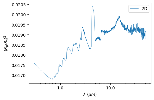
2D day-night transition (transmission)
A simple 2D temperature with a linear transition between the dayside and the nightside can be set up using:
[16]:
temperature = dict(T_day=3300, T_night=500, T_deep=2500, beta=10, p_iso=1e4)
Since the model is not 1D anymore, we need to add latitudes and longitudes to the atmospheric grid. Let us also add more angular points in the grid of rays:
[17]:
input_atmosphere = p3.InputAtmosphere(grid=p3.Grid3D(n_latitudes = 49, n_longitudes = 64),
     temperature = temperature,
     max_pressure = 1e6, min_pressure = 1e-4,
     gas_mix_ratio = {"H2O":5.01187234e-04,
                      "CO2":4.4e-4,
                      "H2":"background"
                     },
     transparent_gases = "H2")

model2 = p3.Model(n_vertical = 100,
     planet=planet,
     star=star,
     orbit=orbit,
     observer=observer,
     input_atmosphere=input_atmosphere,
     transmission=p3.Transmission(rays=p3.Rays(n_radial=100, n_angular=40)),
     opacity=opacity,
     )
Then the model has to be recomputed from scratch:
[18]:
model2.build()
model2.run()
Of course, you can also visualize this spectrum using:
[19]:
plot2 = p3.Plot(model=model2, label="2D", interactive=True, # to show the picture (in addition to saving it)
                out_folder="outputs")
plot2.plot_spectrum()
Saved to `outputs/spectrum_pytmosph3r.pdf`
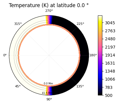
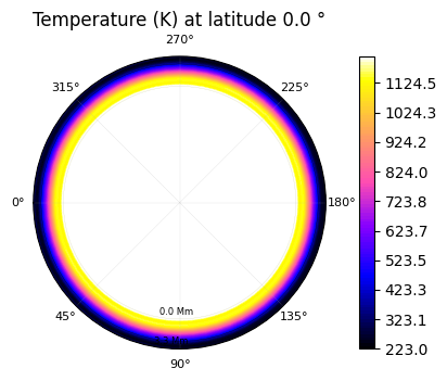
You can check the 2D varations of the temperature using:
[20]:
plot2.t_maps(latitudes=["equator"])
Saved to `outputs/t_map_latitude_24_pytmosph3r.pdf`
Compare models
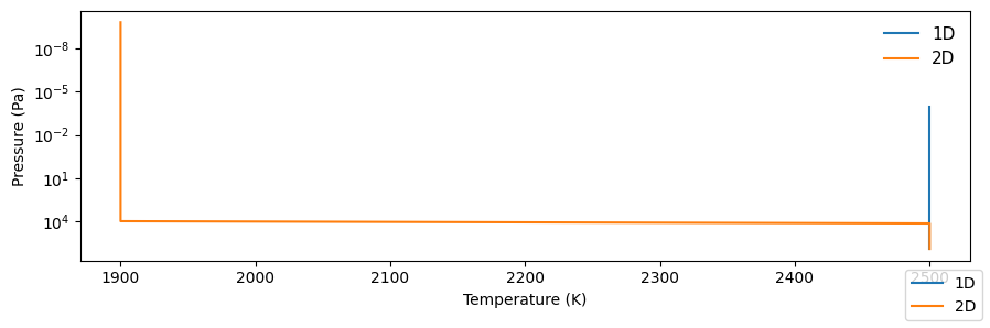
If you have run multiple models (here, the simple 1D and 2D cases above), you can compare them with the following:
[21]:
comparison = p3.plot.Comparison([plot, plot2], interactive=True, out_folder="outputs")
# comparison.diff_spectra(mode='transmission')
comparison.latitudes=["equator"]
comparison.plot_tp()
Saved to `outputs/tp_comp_output.pdf`
GCM Transmission
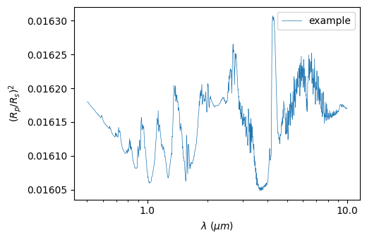
To provide an input file to Pytmosph3R (here “doc/example.nc”), the DiagfiModel and HDF5Model can be used, for netCDF diagfi and HDF5 files, respectively. The input atmosphere can be modified (for example here we set the molecular abundances of \(H_2O\), \(CO_2\) and \(H_2\)):
[22]:
diagfi_file = (data_path / 'gcm' / 'K2-18b_diagfi.nc').as_posix()

input_atmosphere = p3.InputAtmosphere(gas_mix_ratio = {'H2O':5e-4, 'CO2':4.4e-4, "H2":"background"},
                                      transparent_gases = "H2", min_pressure=1e-4)

model = p3.DiagfiModel(n_vertical = 100,
     filename=diagfi_file,
     planet=planet,
     star=star,
     orbit=orbit,
     observer=observer,
     input_atmosphere=input_atmosphere,
     transmission=p3.Transmission(rays=p3.Rays(n_radial=100, n_angular=40)),
     opacity=p3.Opacity(rayleigh=True, cia=['H2', 'He'], wn_range=[1000, 20000]),
     )

model.build()
model.run()
be careful: ()
            String filters not specific enough, several corresponding files have been found.
            We will use the first one:
            /builds/jleconte/pytmosph3r-public/data/corrk/H2O_R300_0.3-50mu.ktable.SI.h5
            Other files are:
            ['/builds/jleconte/pytmosph3r-public/data/corrk/H2O_R300_0.3-50mu.ktable.TauREx.h5']
It is recommended to add a transparent background gas (using the parameter transparent_gases to InputAtmosphere), as has been done for \(H_2\) here.
As before, we can plot the spectrum:
[23]:
plot = p3.Plot(model=model, label="example", interactive=True, out_folder="outputs")
plot.plot_spectrum()
Saved to `outputs/spectrum_pytmosph3r.pdf`
GCM Emission
We give here a full example of an emission spectrum and phase curve generated for a GCM simulation (netCDF format).
[24]:
Rp = 1.807 * 6.9911e7
g0 = 6.67384e-11 * 1.183 * 1.898e27 / Rp**2

input_atmosphere = p3.InputAtmosphere(gas_mix_ratio = {'H2O':5e-4, 'CO2':4.4e-4, "H2":"background"},
                                      transparent_gases = "H2", min_pressure=1e-4)

model = p3.DiagfiModel(n_vertical = 100, input_atmosphere=input_atmosphere,
       filename=diagfi_file,

       planet = p3.Planet(surface_gravity=g0, radius=Rp),
       star = p3.star.Star.fromSolar(temperature=6460.0, radius=1.458), # radius is in sun radii
       orbit=orbit,
       observer=p3.Observer(0, 0),

       # emission=p3.Emission(
       #     planet_to_star_flux_ratio=True, # if you want to normalize to stellar flux
       #     n_phases=20, # activates phase curve
       #     surface_resolution=500, # High resolution increases accuracy (and slowness!)
       # ),
       phasecurve=p3.Phasecurve(n_phases=20),
       opacity=p3.Opacity(rayleigh=True, cia=['H2', 'He'], wn_range=[1000, 20000]),
       )

model.build()
model.run()
be careful: ()
            String filters not specific enough, several corresponding files have been found.
            We will use the first one:
            /builds/jleconte/pytmosph3r-public/data/corrk/H2O_R300_0.3-50mu.ktable.SI.h5
            Other files are:
            ['/builds/jleconte/pytmosph3r-public/data/corrk/H2O_R300_0.3-50mu.ktable.TauREx.h5']
Plots include the phase curves shown for a set of wavelengths, for all wavelengths, and you can also choose to plot a spectrum at a specific phase:
[25]:
plot = p3.Plot(model=model, interactive=True,
               substellar_longitude=0, # longitude of the substellar point (to plot in orbital phases)
               out_folder="outputs")

plot.plot_spectrum(mode='phasecurve', phase=[0,90,180])

plot.plot_phasecurve(wl=[1,8,15])
plot.plot_2d_phasecurve()
Saved to `outputs/spectrum_phasecurve_pytmosph3r.pdf`
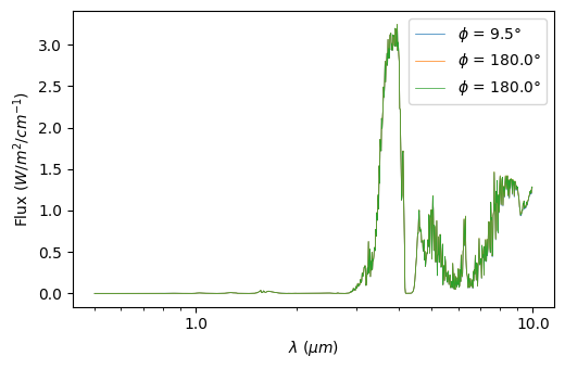
Saved to `outputs/phasecurve_pytmosph3r.pdf`
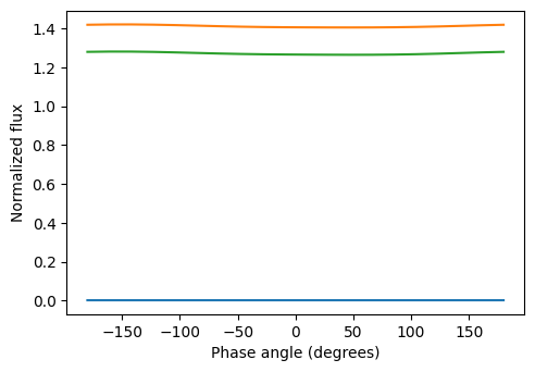
Saved to `outputs/phasecurves_pytmosph3r.pdf`
[25]:
<matplotlib.collections.QuadMesh at 0x7fca55415390>
Gas & aerosols
In our previous examples, the molecular abundances have been set to a constant value. To use more sophisticated profiles, you can use a chemistry module:
[26]:
chemistry = p3.Parmentier2018Dissociation(gases=["H2O"])
Be sure to check the documentation on each chemistry module before using it.
Note
You can also write your own module. For that, try to make a copy of one of the existing chemistries, and change compute_vmr() to set your rules for setting a volume mixing ratio.
You can also use abundances from your input file.
Since your variables may have names that do not correspond to what Pytmosph3R expects, Model has two dictionary parameters gas_dict and aerosol_dict that may be used to specify which name is associated with what gas.
For example,
[27]:
gas_dict = {"H2O": "h2o_var","CO2":"co2_var"}
leads to the variable called h2o_var in the input file (typically a GCM diagfi netCDF file) to be associated with the volume mixing ratio of \(H_2O\), while co2_var will be attributed to \(CO_2\).
Note
The gas_mix_ratio defined in input_atmosphere override the values read from the input file in gas_dict. If a gas was not present in the input file, its value in gas_mix_ratio simply adds it to the composition of the atmosphere.
You can use the gas_units parameter to set the unit of gases (‘mmr’, ‘vmr’, ‘log_vmr’, …).
Note
If your data is MMR and if the input file does not have a ‘controle’ variable in which the molar mass of the gases is stored, you will need to set yourself, to convert the data from MMR to VMR. This is done by setting input_mu to the desired value.
Aerosols are handled via a dictionary similar to the gas one, except that aerosols have also other parameters, such as the effective radius, denoted by reff (see aerosols). See below an example:
[28]:
aerosols_dict = {"H2O":"h2o_ice","H2O_reff":"H2Oice_reff"}
Here h2o_ice is associated with the mass mixing ratio of \(H_2O\) (once again!), but H2Oice_reff to the effective radius of \(H_2O\). The rest of the parameters should be filled in too, and existing ones can be overridden in the InputAtmosphere:
[29]:
aerosols = {'H2O':{'reff':1e-5,'condensate_density':940}}
To create a layer of aerosols below a specific pressure, you could set the mass mixing ratio of the aerosol to a high value:
[30]:
aerosols = {'H2O':{"mmr":1e-1, # in kg/kg
                   "reff":1e-5, # (in m)
                   "condensate_density":940, # in kg/m^3
                   "p_min":1000, # in Pa
                  }}
We give below a full example to create a layer of aerosols:
[31]:
input_atmosphere = p3.InputAtmosphere(gas_mix_ratio={"H2": "background"},
                                      chemistry=p3.InterpolationChemistry(gases=["H2O", "CO2"],
                                                                          filename=str(
                                                                              data_path / "chemistry" / "Parmentier_Abundances-TiO.dat")),
                                      aerosols={'H2O': {"mmr": 1e-1,  # in kg/kg
                                                        "reff": 1e-5,  # (in m)
                                                        "condensate_density": 940,  # in kg/m^3
                                                        "p_min": 1000,  # in Pa
                                                        'optical_properties': 'h2o_ice',
                                                        }},
                                      transparent_gases="H2",
                                      min_pressure=1e-4)

model = p3.DiagfiModel(n_vertical = 100,
    filename=diagfi_file,
    gas_dict = {"H2O": "h2o_var","CO2":"co2_var"},
    aerosols_dict = {"H2O":"h2o_ice","H2O_reff":"H2Oice_reff"},
    planet=planet,
    star=star,
    orbit=orbit,
    observer=observer,
    input_atmosphere=input_atmosphere,
    transmission=p3.Transmission(store_transmittance = True, # to plot transmittance
        rays=p3.Rays(n_radial=100, n_angular=40)),
    opacity=p3.Opacity(rayleigh=True, cia=['H2', 'He'], wn_range=[1000, 20000]))

model.build()
model.run()
/builds/jleconte/pytmosph3r-public/pytmosph3r/util/util.py:218: UserWarning: Unable to determine the kind of log. `units` should be set to `log` or `ln`, provided: `None`.
  warnings.warn(f'Unable to determine the kind of log. `units` should be set to `log` or `ln`, provided: `{units}`.')
be careful: ()
            String filters not specific enough, several corresponding files have been found.
            We will use the first one:
            /builds/jleconte/pytmosph3r-public/data/corrk/H2O_R300_0.3-50mu.ktable.SI.h5
            Other files are:
            ['/builds/jleconte/pytmosph3r-public/data/corrk/H2O_R300_0.3-50mu.ktable.TauREx.h5']
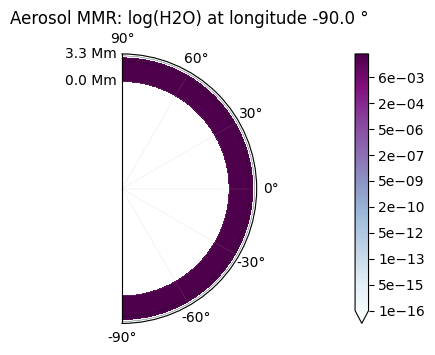
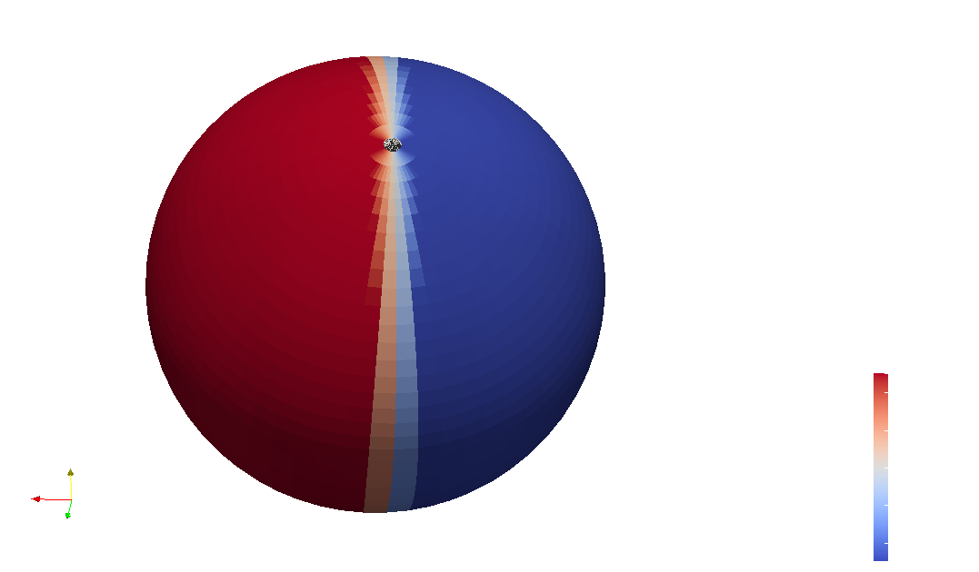
You can check that this layer of aerosols is completely opaque by comparing the map of the aerosol to the transmittance:
[32]:
plot = p3.Plot(model=model, r_factor=0.1, # Rp = Rp/10 to enlarge the atmosphere
               interactive=True, out_folder="outputs")
plot.transmittance_map()
plot.a_maps(["H2O"], longitudes=["terminator"])
/builds/jleconte/pytmosph3r-public/pytmosph3r/plot/modelplot.py:789: UserWarning: set_ticklabels() should only be used with a fixed number of ticks, i.e. after set_ticks() or using a FixedLocator.
  ax.set_xticklabels(["0°","45°","90°","135","180°","225°","270°","315°"], fontsize=9)
Saved to `outputs/transmittances/transmittance_pytmosph3r.pdf`
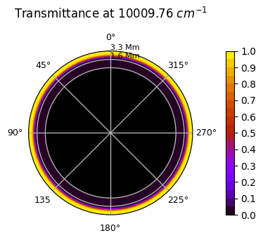
Saved to `outputs/H2O/a_map_longitude_16.pdf`
Other possible plots
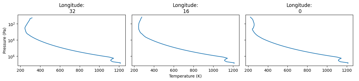
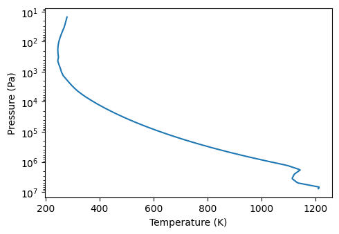
Other types of data can be plotted. For example the PT-profile at three points on the equator may be plotted with this command:
[33]:
plot.latitudes=["equator"]
plot.longitudes=["day", "terminator", "night"]
plot.plot_tps()
No artists with labels found to put in legend. Note that artists whose label start with an underscore are ignored when legend() is called with no argument.
Saved to `outputs/tp_pytmosph3r.pdf`
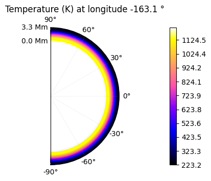
The temperature can be represented as a 2D colormap if a specific altitude is chosen (or latitude, or longitude).
[34]:
plot.t_maps(altitudes=["middle"]) #other possibilities: "top", "surface" or the layer index
plot.t_maps(latitudes=["equator"])
plot.t_maps(longitudes=["day", 3])
Saved to `outputs/t_map_altitude_50_pytmosph3r.pdf`
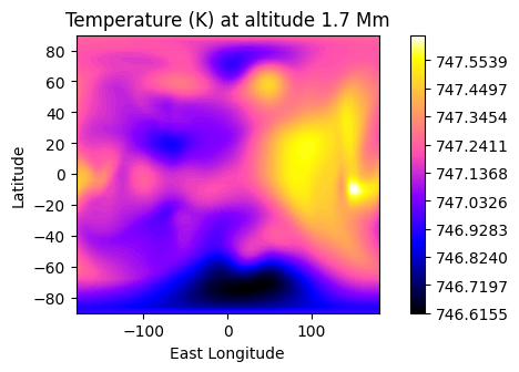
Saved to `outputs/t_map_latitude_24_pytmosph3r.pdf`
Saved to `outputs/t_map_longitude_32_pytmosph3r.pdf`
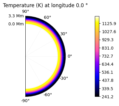
Saved to `outputs/t_map_longitude_3_pytmosph3r.pdf`
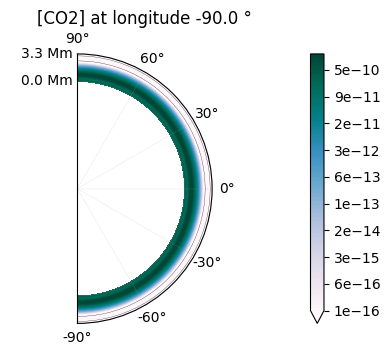
2D maps of the molecular distribution are also possible:
[35]:
plot.x_maps(["H2O", "CO2"], altitudes=["middle"])
plot.x_maps(["H2O", "CO2"], latitudes=["equator"])
plot.x_maps(["H2O", "CO2"], longitudes=["terminator"])
Saved to `outputs/H2O/H2O_map_altitude_50_pytmosph3r.pdf`
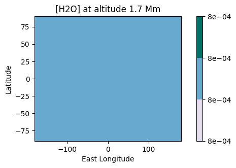
Saved to `outputs/CO2/CO2_map_altitude_50_pytmosph3r.pdf`
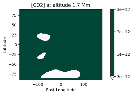
Saved to `outputs/H2O/H2O_map_latitude_24_pytmosph3r.pdf`
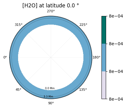
Saved to `outputs/CO2/CO2_map_latitude_24_pytmosph3r.pdf`
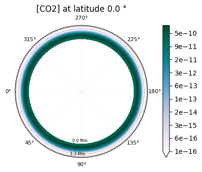
Saved to `outputs/H2O/H2O_map_longitude_16_pytmosph3r.pdf`
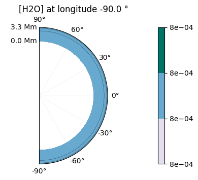
Saved to `outputs/CO2/CO2_map_longitude_16_pytmosph3r.pdf`
Note
For more information on all available plots, see Plot. If you encounter some problems, you can debug the library by running in debug mode (use p3.debug()).
Output files
The model can be saved using the HDF5 format to have maximum information. But to be able to visualize the data with softwares such as ncview or ParaView, you also have the option of writing a netCDF file.
netCDF
To visualize the atmopshere using paraview or ncview, you can save the model in a netCDF format using:
[36]:
p3.interface.write_netcdf("outputs/output_tutorial.nc", model)
You can check the header of the netCDF with ncdump:
[37]:
!ncdump -h "outputs/output_tutorial.nc"
/usr/bin/sh: 1: ncdump: not found
In paraview, you will be able to see something like this:
HDF5
Writing an output HDF5 file
To save the model using the HDF5 format, we recommend to split the output in two parts. The first part is the model with its “input” parameters so that one can re-run Pytmosph3R using this file. This can be done by running the following piece of code preferably before running the model (but after building it with build()).
[38]:
p3.write_hdf5("outputs/output_tutorial.h5", model, "Model")
In case running the model fails, you will at least have the input model saved somewhere to investigate where the error might come from.
Once you have run the model (with run()), you can save its outputs in the “Output” group:
[39]:
p3.write_hdf5("outputs/output_tutorial.h5", model, "Output")
Following the division “Model” and “Output” is advised to be able to re-use the file for a new run or for plots.
Alternatively, you can also write the inputs and outputs using:
[40]:
p3.write_hdf5("outputs/output_tutorial.h5", model, "All")
Reading a HDF5 (pytmosph3r) file
The HDF5 output file can be read with Plot() to make various plots.
You can also reload a model, change its parameters and re-run it:
[41]:
# Plotting the hdf5 output
plot = p3.Plot("outputs/output_tutorial.h5", interactive=True, out_folder='outputs')
plot.plot_tp() # initial temperature profile in the simulation

# reloading the hdf5 output
f = p3.HDF5Input("outputs/output_tutorial.h5")
model = f.read('Model')
model.build()
No artists with labels found to put in legend. Note that artists whose label start with an underscore are ignored when legend() is called with no argument.
Saved to `outputs/tp_north_day_pytmosph3r.pdf`
/builds/jleconte/pytmosph3r-public/pytmosph3r/util/util.py:218: UserWarning: Unable to determine the kind of log. `units` should be set to `log` or `ln`, provided: `None`.
  warnings.warn(f'Unable to determine the kind of log. `units` should be set to `log` or `ln`, provided: `{units}`.')
[42]:
model.input_atmosphere.temperature = 2500 # overwrite temperature

model.build()
[43]:
# model.run()
plot = p3.Plot(model=model, interactive=True, out_folder='outputs')
plot.plot_tp() # new temperature profile
No artists with labels found to put in legend. Note that artists whose label start with an underscore are ignored when legend() is called with no argument.
Saved to `outputs/tp_north_day_pytmosph3r.pdf`